PDE/ODE Solvers
Runge Kutta Method
The Runge Kutta method is one of the workhorses for solving ODEs. The method is a higher order interpolation to the derivatives. The system of ODE has the form
\[\frac{dy}{dt} = f(y, t, \theta)\]
where $t$ denotes time, $y$ denotes states and $\theta$ denotes parameters.
The Runge-Kutta method is defined as
\[\begin{aligned} k_1 &= \Delta t f(t_n, y_n, \theta)\\ k_2 &= \Delta t f(t_n+\Delta t/2, y_n + k_1/2, \theta)\\ k_3 &= \Delta t f(t_n+\Delta t/2, y_n + k_2/2, \theta)\\ k_4 &= \Delta t f(t_n+\Delta t, y_n + k_3, \theta)\\ y_{n+1} &= y_n + \frac{k_1}{6} +\frac{k_2}{3} +\frac{k_3}{3} +\frac{k_4}{6} \end{aligned}\]
ADCME provides a built-in Runge Kutta solver rk4 and ode45. Consider an example: the Lorentz equation
\[\begin{aligned} \frac{dx}{dt} &= 10(y-x)\\ \frac{dy}{dt} &= x(27-z)-y\\ \frac{dz}{dt} &= xy -\frac{8}{3}z \end{aligned}\]
Let the initial condition be $x_0 = [1,0,0]$, the following code snippets solves the Lorentz equation with ADCME
function f(t, y, θ)
    [10*(y[2]-y[1]);y[1]*(27-y[3])-y[2];y[1]*y[2]-8/3*y[3]]
end
x0 = [1.;0.;0.]
rk4(f, 30.0, 10000, x0)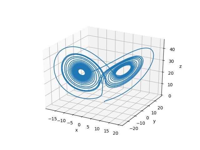
We can also solve three body problem with the Runge-Kutta method. The full script is
#
# adapted from
# https://github.com/pjpmarques/Julia-Modeling-the-World/
#
using Revise
using ADCME
using PyPlot
using Printf

function f(t, y, θ)
    # Extract the position and velocity vectors from the g array
    r0, v0 = y[1:2], y[3:4]
    r1, v1 = y[5:6], y[7:8]
    r2, v2 = y[9:10], y[11:12]

    # The derivatives of the position are simply the velocities
    dr0 = v0
    dr1 = v1
    dr2 = v2

    # Now calculate the the derivatives of the velocities, which are the accelarations
    # Start by calculating the distance vectors between the bodies (assumes m0, m1 and m2 are global variables)
    # Slightly rewriten the expressions dv0, dv1 and dv2 comprared to the normal equations so we can reuse d0, d1 and d2
    d0  = (r2 - r1) / ( norm(r2 - r1)^3.0 )
    d1  = (r0 - r2) / ( norm(r0 - r2)^3.0 )
    d2  = (r1 - r0) / ( norm(r1 - r0)^3.0 )

    dv0 = m1*d2 - m2*d1
    dv1 = m2*d0 - m0*d2
    dv2 = m0*d1 - m1*d0

    # Reconstruct the derivative vector
    [dr0; dv0; dr1; dv1; dr2; dv2]
end

function plot_trajectory(t1, t2)

    t1i = round(Int,NT * t1/T) + 1
    t2i = round(Int,NT * t2/T) + 1

    # Plot the initial and final positions
    # In these vectors, the first coordinate will be X and the second Y
    X = 1
    Y = 2

    # figure(figsize=(6,6))
    plot(r0[t1i,X], r0[t1i,Y], "ro")
    plot(r0[t2i,X], r0[t2i,Y], "rs")
    plot(r1[t1i,X], r1[t1i,Y], "go")
    plot(r1[t2i,X], r1[t2i,Y], "gs")
    plot(r2[t1i,X], r2[t1i,Y], "bo")
    plot(r2[t2i,X], r2[t2i,Y], "bs")

    # Plot the trajectories
    plot(r0[t1i:t2i,X], r0[t1i:t2i,Y], "r-")
    plot(r1[t1i:t2i,X], r1[t1i:t2i,Y], "g-")
    plot(r2[t1i:t2i,X], r2[t1i:t2i,Y], "b-")

    # Plot cente of mass
    # plot(cx[t1i:t2i], cy[t1i:t2i], "kx")

    # Setup the axis and titles
    xmin = minimum([r0[t1i:t2i,X]; r1[t1i:t2i,X]; r2[t1i:t2i,X]]) * 1.10
    xmax = maximum([r0[t1i:t2i,X]; r1[t1i:t2i,X]; r2[t1i:t2i,X]]) * 1.10
    ymin = minimum([r0[t1i:t2i,Y]; r1[t1i:t2i,Y]; r2[t1i:t2i,Y]]) * 1.10
    ymax = maximum([r0[t1i:t2i,Y]; r1[t1i:t2i,Y]; r2[t1i:t2i,Y]]) * 1.10

    axis([xmin, xmax, ymin, ymax])
    title(@sprintf "3-body simulation for t=[%.1f .. %.1f]" t1 t2)
end;

m0 = 5.0
m1 = 4.0
m2 = 3.0

# Initial positions and velocities of each body (x0, y0, vx0, vy0)
gi0 = [ 1.0; -1.0; 0.0; 0.0]
gi1 = [ 1.0;  3.0; 0.0; 0.0]
gi2 = [-2.0; -1.0; 0.0; 0.0]


T  = 30.0
NT  = 500*300
g0  = [gi0; gi1; gi2]

res_ = ode45(f, T, NT, g0)

sess = Session(); init(sess)
res = run(sess, res_)

r0, v0, r1, v1, r2, v2 = res[:,1:2], res[:,3:4], res[:,5:6], res[:,7:8], res[:,9:10], res[:,11:12]

figure(figsize=[4,1])
subplot(131); plot_trajectory(0.0,10.0)
subplot(132); plot_trajectory(10.0,20.0)
subplot(133); plot_trajectory(20.0,30.0)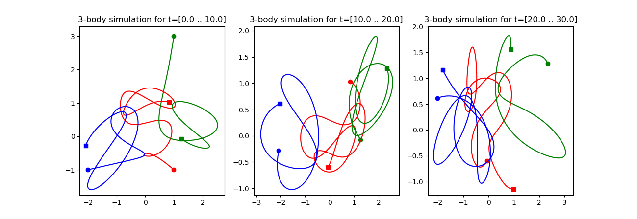
Explicit Newmark Scheme
ExplicitNewmark provides an explicit Newmark integrator for
\[M \ddot{\mathbf{d}} + Z_1 \dot{\mathbf{d}} + Z_2 \mathbf{d} + f = 0\]
The numerical scheme is given by
\[\left(\frac{1}{\Delta t^2} M + \frac{1}{2\Delta t}Z_1\right)d^{n+1} = \left(\frac{2}{\Delta t^2} M - \frac{1}{2\Delta t}Z_2\right)d^n - \left(\frac{1}{\Delta t^2} M - \frac{1}{2\Delta t}Z_1\right) d^{n-1} - f^n\]
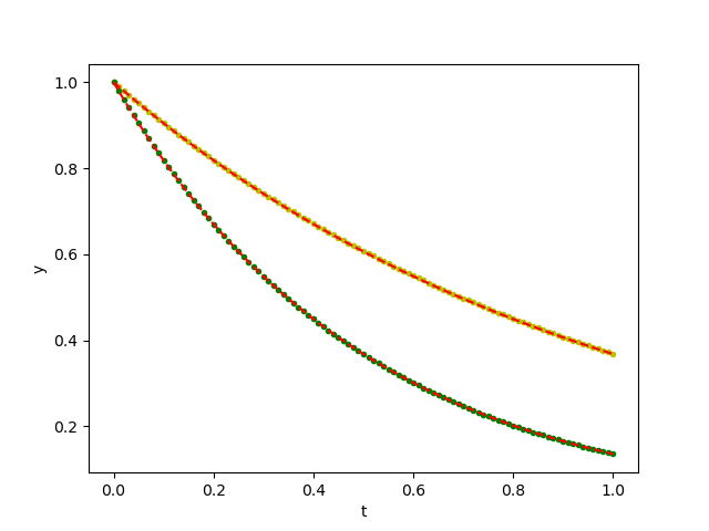
We consider an example:
\[\mathbf{d} = \begin{bmatrix}e^{-t}\\ e^{-2t}\end{bmatrix}\]
and
\[M = \begin{bmatrix}1 & 2\\3 &4 \end{bmatrix}\qquad Z_1 = \begin{bmatrix}5 & 6\\7 &8 \end{bmatrix}\qquad Z_2 =\begin{bmatrix}9 & 10\\11 &12 \end{bmatrix}\]
The function $f$ is given by
\[f(t) = -\begin{bmatrix}5e^{-t} + 6e^{-2t}\\ 7 e^{-t} + 12 e^{-2t}\end{bmatrix}\]
We can carry out the simulation using the following codes:
using ADCME
using PyPlot

M = Float64[1 2;3 4]
Z1 = Float64[5 6;7 8]
Z2 = Float64[9 10;11 12]

NT = 200
Δt = 1/NT

F = zeros(NT+1, 2)
for i = 1:NT+1
    t = (i-1)*Δt
    F[i,1] = -(5exp(-t) + 6exp(-2t))
    F[i,2] = -(7exp(-t) + 12exp(-2t))
end
F = constant(F)

en = ExplicitNewmark(M, Z1, Z2, Δt)

function condition(i, d)
    i<=NT
end

function body(i, d)
    d0 = read(d, i-1)
    d1 = read(d, i)
    d2 = step(en, d0, d1, F[i-1])
    i+1, write(d, i+1, d2)
end

d = TensorArray(NT+1)
d = write(d, 1, [1.0;1.0])
d = write(d, 2, [exp(-Δt);exp(-2Δt)])
i = constant(2, dtype = Int32)
_, d = while_loop(condition, body, [i, d])
d = stack(d)

sess = Session(); init(sess)
D = run(sess, d)
ts = (0:NT)*Δt
close("all")
plot(ts, D[:, 1], "b.")
plot(ts, D[:,2], "g.")
plot(ts, exp.(-ts), "r--")
plot(ts, exp.(-2ts), "r--")
xlabel("t"); ylabel("y")
savefig("ode_solution.png")
Newmark Algorithm
Besides the explicit Newmark algorithm, we also provide the a-form Newmark algorithm: Newmark. It is a time integrator for
\[M\ddot \mathbf{d} + C \dot\mathbf{d} + K \mathbf{d} + f = 0\]
The numerical scheme is given by
\[\begin{aligned} \tilde d_{n+1} &= d_n + \Delta t v_n + \Delta^2/2(1-2\beta)a_n \\ \tilde v_{n+1} &= v_n + (1-\gamma)\Delta a_n \\ (M+\gamma\Delta C+\beta \Delta^2 K)a_{n+1} &= F_{n+1} - C\tilde v_{n+1} - K\tilde d_{n+1}\\ d_{n+1} &= \tilde d_{n+1} + \beta \Delta^2 a_{n+1}\\ v_{n+1} &= \tilde v_{n+1} + \gamma \Delta ta_n \end{aligned}\]
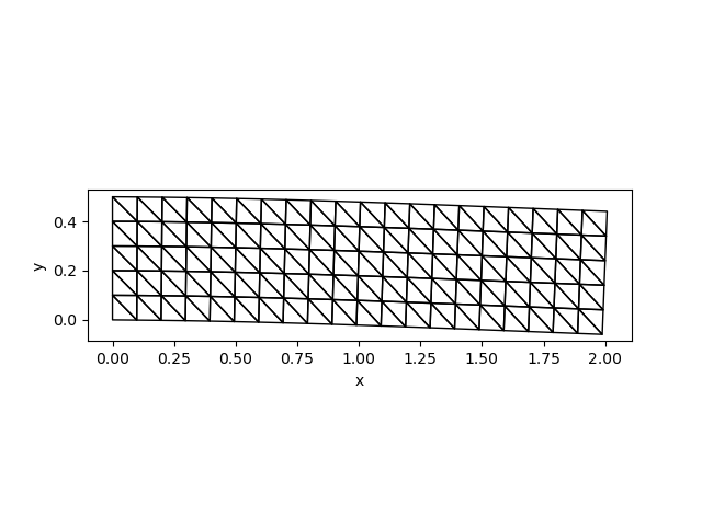
Let us consider an example. The left side of the beam is fixed, while the other boundaries are considered free surface. The beam is subject to the gravity force. The governing equation for interior points are
\[\rho\ddot u = \mathrm{div} \sigma + f\]
The constitutive law is given by
\[\sigma_{ij} = C_{ijlk} \epsilon_{lk},\quad \epsilon = \frac12\left(\nabla u + (\nabla u)^T\right)\]
We use a plane stress linear elasticity model with $E = 1000.0, \nu = 0.3$.
Using AdFem, the code is as follows
using AdFem

mmesh = Mesh(20, 5, 0.1)
NT = 100
Δt = 0.3/NT
bd = bcnode((x,y)->x<0.001, mmesh)
M = compute_fem_mass_matrix(ones(get_ngauss(mmesh)), mmesh)
H = compute_plane_stress_matrix(1000.0, 0.3)
K = compute_fem_stiffness_matrix(H, mmesh)
F = compute_fem_source_term(ones(get_ngauss(mmesh)), ones(get_ngauss(mmesh)), mmesh)
nm = Newmark(M, spzero(2mmesh.ndof), K, Δt, factorize_S = false)
Now we need to impose the boundary condition. To this end, since we have a fixed Dirichlet boundary condition, all we need to do is to ensure that the left boundary component of the acceleration $a$ is zero.
nm.S, F = impose_Dirichlet_boundary_conditions(nm.S, F, [bd; bd .+ mmesh.ndof], zeros(2length(bd)))
nm.S = factorize(nm.S)
nm.C = impose_Dirichlet_boundary_conditions(nm.C, [bd; bd .+ mmesh.ndof])
nm.K = impose_Dirichlet_boundary_conditions(nm.K, [bd; bd .+ mmesh.ndof])
Now we can carry out the simulation
d = TensorArray(NT+1)
v = TensorArray(NT+1)
a = TensorArray(NT+1)

d = write(d, 1, zeros(2mmesh.ndof))
v = write(v, 1, zeros(2mmesh.ndof))
a = write(a, 1, zeros(2mmesh.ndof))
i = constant(2, dtype = Int32)

function condition(i, ta...)
    i<=NT+1
end


function body(i, ta...)
    d, v, a = ta
    d0, v0, a0 = step(nm, read(d, i-1), read(v, i-1), read(a, i-1), F)
    i+1, write(d, i, d0), write(v, i, v0), write(a, i, a0)
end

_, darr, varr, aarr = while_loop(condition, body, [i, d, v, a])

D, V, A = stack(darr), stack(varr), stack(aarr)

sess = Session(); init(sess)
Darr, Varr, Aarr = run(sess, [D, V, A])


close("all")
visualize_displacement(Darr[end,:], mmesh)
savefig("newmark_simple.png")
The solution at $t=0.3$ is as follows:
 Complete Code
using AdFem

mmesh = Mesh(20, 5, 0.1)
NT = 100
Δt = 0.3/NT
bd = bcnode((x,y)->x<0.001, mmesh)
M = compute_fem_mass_matrix(ones(get_ngauss(mmesh)), mmesh)
H = compute_plane_stress_matrix(1000.0, 0.3)
K = compute_fem_stiffness_matrix(H, mmesh)
F = compute_fem_source_term(ones(get_ngauss(mmesh)), ones(get_ngauss(mmesh)), mmesh)
nm = Newmark(M, spzero(2mmesh.ndof), K, Δt, factorize_S = false)

nm.S, F = impose_Dirichlet_boundary_conditions(nm.S, F, [bd; bd .+ mmesh.ndof], zeros(2length(bd)))
nm.S = factorize(nm.S)
nm.C = impose_Dirichlet_boundary_conditions(nm.C, [bd; bd .+ mmesh.ndof])
nm.K = impose_Dirichlet_boundary_conditions(nm.K, [bd; bd .+ mmesh.ndof])

d = TensorArray(NT+1)
v = TensorArray(NT+1)
a = TensorArray(NT+1)

d = write(d, 1, zeros(2mmesh.ndof))
v = write(v, 1, zeros(2mmesh.ndof))
a = write(a, 1, zeros(2mmesh.ndof))
i = constant(2, dtype = Int32)

function condition(i, ta...)
    i<=NT+1
end


function body(i, ta...)
    d, v, a = ta
    d0, v0, a0 = step(nm, read(d, i-1), read(v, i-1), read(a, i-1), F)
    i+1, write(d, i, d0), write(v, i, v0), write(a, i, a0)
end

_, darr, varr, aarr = while_loop(condition, body, [i, d, v, a])

D, V, A = stack(darr), stack(varr), stack(aarr)

sess = Session(); init(sess)
Darr, Varr, Aarr = run(sess, [D, V, A])


close("all")
visualize_displacement(Darr[end,:], mmesh)
savefig("explicit_newmark.png")
Calculating Initial Acceleration
Consider another scenario: there is a small slip on the right hand side at $t=0$ and both left and right sides are fixed thereafter.
using AdFem
using PyPlot

mmesh = Mesh(20, 5, 0.1)
NT = 100
Δt = 0.3/NT
bd = bcnode((x,y)->x<0.001, mmesh)
bdr = bcnode((x,y)->x>2-0.001, mmesh)
M = compute_fem_mass_matrix(ones(get_ngauss(mmesh)), mmesh)
H = compute_plane_stress_matrix(1000.0, 0.3)
K = compute_fem_stiffness_matrix(H, mmesh)
F = zeros(2mmesh.ndof)
nm = Newmark(M, spzero(2mmesh.ndof), K, Δt, factorize_S = false)

bd_ = [bd; bdr; bd .+ mmesh.ndof; bdr .+ mmesh.ndof]
nm.S = impose_Dirichlet_boundary_conditions(nm.S, bd_)
nm.S = factorize(nm.S)
nm.C = impose_Dirichlet_boundary_conditions(nm.C, bd_)
nm.K = zero_out_row(nm.K, bd_)

d = TensorArray(NT+1)
v = TensorArray(NT+1)
a = TensorArray(NT+1)

d0 = zeros(2mmesh.ndof)
d0[bdr.+mmesh.ndof] .= 0.5 * 0.1
d = write(d, 1, d0)
v = write(v, 1, zeros(2mmesh.ndof))
a0 = nm.S\(-nm.K * d0)
a = write(a, 1, a0)
i = constant(2, dtype = Int32)

function condition(i, ta...)
    i<=NT+1
end


function body(i, ta...)
    d, v, a = ta
    d0, v0, a0 = step(nm, read(d, i-1), read(v, i-1), read(a, i-1), F)
    i+1, write(d, i, d0), write(v, i, v0), write(a, i, a0)
end

_, darr, varr, aarr = while_loop(condition, body, [i, d, v, a])

D, V, A = stack(darr), stack(varr), stack(aarr)

sess = Session(); init(sess)
Darr, Varr, Aarr = run(sess, [D, V, A])


close("all")
function update(i)
    clf()
    visualize_displacement(Darr[i,:], mmesh)
end
p = animate(update, 1:NT)
saveanim(p, "initial_acce.gif")
Build Your Own Solvers
Sometimes it is helpful to build your own ODE/PDE solvers. The basic routine is
- Implement the one step state transition function;
- Use
while_loopto build the time integrator.
As an example, we build a second-order Runge-Kutta scheme for
\[\dot{\mathbf{d}} + \beta \mathbf{d} = \mathbf{t}\]
The numerical scheme is
\[\begin{aligned}h_1 &= -\beta \mathbf{d}^n + \mathbf{t}^n\\ h_2 &= -\beta(\mathbf{d}^n + \Delta t h_1) + \mathbf{t}^n\\ \mathbf{d}^{n+1} &= \mathbf{d}^n + \frac{\Delta t}{2}(h_1 + h_2)\end{aligned}\]
The state transition function has the following form
function rk_one_step(d2, t)
    h1 = -β*d2 + t
    h2 = -β*(d2+Δt*h1)+t
    d2 + Δt/2*(h1+h2)
end
Now consider an analytical solution
\[\mathbf{d} = \begin{bmatrix}e^{-t}\\e^{-2t}\end{bmatrix}, \quad \beta = 2\]
Then we have
\[\mathbf{t} = \begin{bmatrix}e^{-t}\\0\end{bmatrix}\]
The main code is as follows
using ADCME
using PyPlot

NT = 100
Δt = 1/NT
ts = Array((0:NT)*Δt)
t = constant([exp.(-ts) zeros(NT+1)])
β = 2.0


function condition(i, d)
    i<=NT
end

function body(i, d)
    d0 = read(d, i)
    d1 = rk_one_step(d0, t[i])
    i+1, write(d, i+1, d1)
end

d = TensorArray(NT+1)
d = write(d, 1, ones(2))
i = constant(1, dtype = Int32)
_, d = while_loop(condition, body, [i, d])
d = stack(d)

sess = Session(); init(sess)
D = run(sess, d)

close("all")
plot(ts, D[:,1], "y.")
plot(ts, D[:,2], "g.")
plot(ts, exp.(-ts), "r--")
plot(ts, exp.(-2ts), "r--")
xlabel("t"); ylabel("y")
savefig("ode_solution2.png")