Inverse Modeling with ADCME
Roughly speaking, there are four types of inverse modeling in partial differential equations. We have developed numerical methods that takes advantage of deep neural networks and automatic differentiation. To be more concrete, let the forward model be a 1D Poisson equation
\[\begin{aligned}-\nabla (X\nabla u(x)) &= \varphi(x) & x\in (0,1)\\ u(0)=u(1) &= 0\end{aligned}\]
Here $X$ is the unknown which may be one of the four forms: parameter, function, functional or random variable.
| Inverse problem | Problem type | ADCME Approach | Reference |
|---|---|---|---|
| $\nabla\cdot(c\nabla u) = \varphi(x)$ | Parameter | Adjoint-State Method | 1 2 |
| $\nabla\cdot(f(x)\nabla u) = \varphi(x)$ | Function | DNN as a Function Approximator | 3 |
| $\nabla\cdot(f(u)\nabla u) = \varphi(x)$ | Functional | Residual Learning or Physics Constrained Learning | 4 |
| $\nabla\cdot(\varpi\nabla u) = \varphi(x)$ | Stochastic Inversion | Generative Neural Networks | 5 |
Parameter Inverse Problem
When $X$ is just a scalar/vector, we call this type of problem parameter inverse problem. We consider a manufactured solution: the exact $X=1$ and $u(x)=x(1-x)$, so we have
\[\varphi(x) = 2\]
Assume we can observe $u(0.5)=0.25$ and the initial guess for $X_0=10$. We use finite difference method to discretize the PDE and the interval $[0,1]$ is divided uniformly to $0=x_0<x_1<\ldots<x_n=1$, with $n=100$, $x_{i+1}-x_i = h=\frac{1}{n}$.
we can solve the problem with the following code snippet
using ADCME
n = 100
h = 1/n
X0 = Variable(10.0)
A = X0 * diagm(0=>2/h^2*ones(n-1), 1=>-1/h^2*ones(n-2), -1=>-1/h^2*ones(n-2)) # coefficient matrix for the finite difference
φ = 2.0*ones(n-1) # right hand side
u = A\φ
loss = (u[50] - 0.25)^2

sess = Session(); init(sess)
BFGS!(sess, loss)
After around 7 iterations, the estimated $X_0$ converges to 1.0000000016917243.
Function Inverse Problem
When $X$ is a function that does not depend on $u$, i.e., a function of location $x$, we call this type of problem function inverse problem. A common approach to this type of problem is to approximate the unknown function $X$ with a parametrized form, such as piecewise linear functions, radial basis functions or Chebyshev polynomials; sometimes we can also discretize $X$ and substitute $X$ by a vector of its values at the discrete grid nodes.
This tutorial is not aimed at the comparison of different methods. Instead, we show how we can use neural networks to represent $X$ and train the neural network by coupling it with numerical schemes. The gradient calculation can be laborious with the traditional adjoint state methods but is trivial with automatic differentiation.
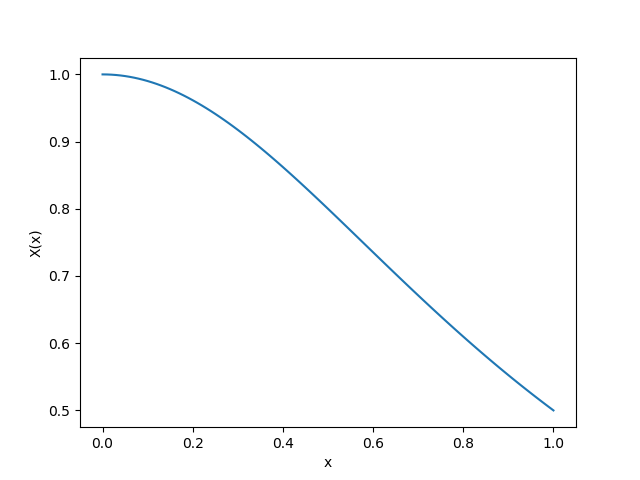
Let's assume the true $X$ has the following form
\[X(x) = \frac{1}{1+x^2}\]
The exact $\varphi$ is given by
\[\varphi(x) = \frac{2 \left(x^{2} - x \left(2 x - 1\right) + 1\right)}{\left(x^{2} + 1\right)^{2}}\]
The idea is to use a neural network $\mathcal{N}(x;w)$ with weights and biases $w$ that maps the location $x\in \mathbb{R}$ to a scalar value such that
\[\mathcal{N}(x; w)\approx X(x)\]
To find the optional $w$, we solve the Poisson equation with $X(x)=\mathcal{N}(x;w)$, where the numerical scheme is
\[\left( -\frac{X_i+X_{i+1}}{2} \right) u_{i+1} + \frac{X_{i-1}+2X_i+X_{i+1}}{2} u_i + \left( -\frac{X_i+X_{i-1}}{2} \right) = \varphi(x_i) h^2\]
Here $X_i = \mathcal{N}(x_i; w)$.
Assume we can observe the full solution $u(x)$, we can compare it with the solution $u(x;w)$, and minimize the loss function
\[L(w) = \sum_{i=2}^{n-1} (u(x_i;w)-u(x_i))^2\]
using ADCME
n = 100
h = 1/n
x = collect(LinRange(0, 1.0, n+1))
X = ae(x, [20,20,20,1])^2  # to ensure that X is positive, we use NN^2 instead of NN
A = spdiag(
  n-1,
  1=>-(X[2:end-2] + X[3:end-1])/2,
  -1=>-(X[3:end-1] + X[2:end-2])/2,
  0=>(2*X[2:end-1]+X[3:end]+X[1:end-2])/2
)/h^2
φ = @. 2*x*(1 - 2*x)/(x^2 + 1)^2 + 2 /(x^2 + 1)
u = A\φ[2:end-1] # for efficiency, we can use A\φ[2:end-1] (sparse solver)
u_obs = (@. x * (1-x))[2:end-1]
loss = sum((u - u_obs)^2)

sess = Session(); init(sess)
BFGS!(sess, loss)
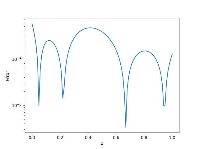
We show the exact $X(x)$ and the pointwise error in the following plots
\[\left|\mathcal{N}(x_i;w)-X(x_i)\right|\]
 |  |
|---|---|
| Pointwise Absolute Error | Exact $X(u)$ |
Functional Inverse Problem
In the functional inverse problem, $X$ is a function that depends on $u$ (or both $x$ and $u$); it must not be confused with the functional inverse problem and it is much harder to solve (since the equation is nonlinear).
As an example, assume
\[\begin{aligned}\nabla (X(u)\nabla u(x)) &= \varphi(x) & x\in (0,1)\\ u(0)=u(1) &= 0\end{aligned}\]
where the quantity of interest is
\[X(u) = \frac{1}{1+100u^2}\]
The corresponding $\varphi$ can be analytically evaluated (e.g., using SymPy).
To solve the Poisson equation, we use the standard Newton-Raphson scheme, in which case, we need to compute the residual
\[R_i = X'(u_i)\left(\frac{u_{i+1}-u_{i-1}}{2h}\right)^2 + X(u_i)\frac{u_{i+1}+u_{i-1}-2u_i}{h^2} - \varphi(x_i)\]
and the corresponing Jacobian
\[\frac{\partial R_i}{\partial u_j} = \left\{ \begin{matrix} -\frac{X'(u_i)}{h}\frac{u_{i+1}-u_{i-1}}{2h} + \frac{X(u_i)}{h^2} & j=i-1\\ X''(u_i)\frac{u_{i+1}-u_{i-1}}{2h} + X'(u_i)\frac{u_{i+1}+u_{i-1}-2u_i}{h^2} - \frac{2}{h^2}X(u_i) & j=i \\ \frac{X'(u_i)}{2h}\frac{u_{i+1}-u_{i-1}}{2h} + \frac{X(u_i)}{h^2} & j=i+1\\ 0 & |j-i|>1 \end{matrix} \right.\]
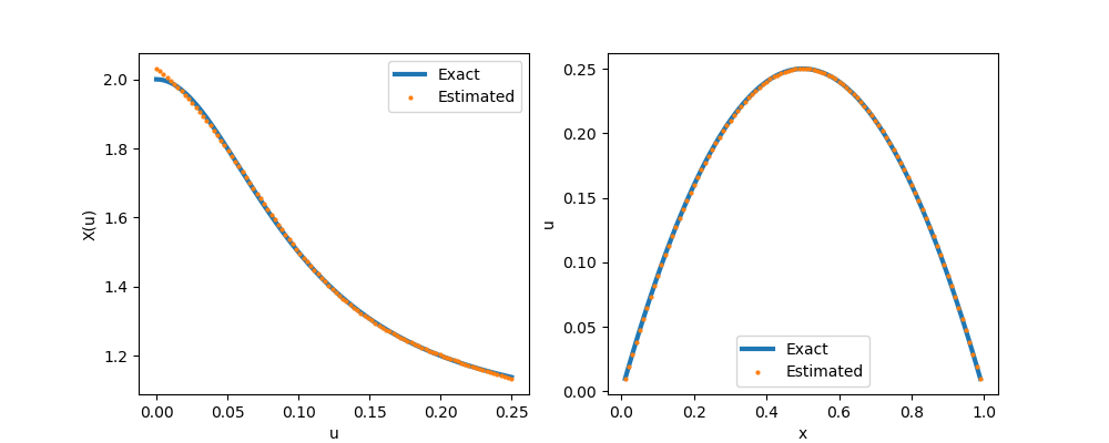
Just like the function inverse problem, we also use a neural network to approximate $X(u)$; the difference is that the input of the neural network is $u$ instead of $x$. It is convenient to compute $X'(u)$ with automatic differentiation.
Solving the forward problem (given $X(u)$, solve for $u$) requires conducting Newton-Raphson iterations. One challenge here is that the Newton-Raphson operator is a nonlinear implicit operator that does not fall into the types of operators where automatic differentiation applies. The relevant technique is physics constrained learning. The basic idea is to extract the gradients by the implicit function theorem. The limitation is that we need to provide the Jacobian matrix for the residual term in the Newton-Raphson algorithm. In ADCME, the complex algorithm is wrapped in the API NonlinearConstrainedProblem and users only need to focus on constructing the residual and the gradient term
using ADCME
using PyPlot

function residual_and_jacobian(θ, u)
    X = ae(u, config, θ) + 1.0     # (1)
    Xp = tf.gradients(X, u)[1]
    Xpp = tf.gradients(Xp, u)[1]
    up = [u[2:end];constant(zeros(1))]
    un = [constant(zeros(1)); u[1:end-1]]
    R = Xp .* ((up-un)/2h)^2 + X .* (up+un-2u)/h^2 - φ
    dRdu = Xpp .* ((up-un)/2h)^2 + Xp.*(up+un-2u)/h^2 - 2/h^2*X
    dRdun = -Xp[2:end]/h .* (up-un)[2:end]/2h + X[2:end]/h^2
    dRdup = Xp[1:end-1]/h .* (up-un)[1:end-1]/2h + X[1:end-1]/h^2
    J = spdiag(n-1,
        -1=>dRdun,
        0=>dRdu,
        1=>dRdup)     # (2)
    return R, J
end


config = [20,20,20,1]
n = 100
h = 1/n
x = collect(LinRange(0, 1.0, n+1))

φ = @. (1 - 2*x)*(-100*x^2*(2*x - 2) - 200*x*(1 - x)^2)/(100*x^2*(1 - x)^2 + 1)^2 - 2 - 2/(100*x^2*(1 - x)^2 + 1)
φ = φ[2:end-1]
θ = Variable(ae_init([1,config...]))
u0 = constant(zeros(n-1))
function L(u)    # (3)
  u_obs = (@. x * (1-x))[2:end-1]
  loss = mean((u - u_obs)^2)
end
loss, solution, grad = NonlinearConstrainedProblem(residual_and_jacobian, L, θ, u0)
X_pred = ae(collect(LinRange(0.0,0.25,100)), config, θ) + 1.0

sess = Session(); init(sess)
BFGS!(sess, loss, grad, θ)
x_pred, sol = run(sess, [X_pred, solution])

figure(figsize=(10,4))
subplot(121)
s = LinRange(0.0,0.25,100)
x_exact = @. 1/(1+100*s^2) + 1
plot(s, x_exact, "-", linewidth=3, label="Exact")
plot(s, x_pred, "o", markersize=2, label="Estimated")
legend()
xlabel("u")
ylabel("X(u)")

subplot(122)
s = LinRange(0.0,1.0,101)[2:end-1]
plot(s, (@. s * (1-s)), "-", linewidth=3, label="Exact")
plot(s, sol, "o", markersize=2, label="Estimated")
legend()
xlabel("x")
ylabel("u")
savefig("nn.png")
Detailed explaination: (1) This is the neural network we constructed. Note that with default initialization, the neural network output values are close to 0, and thus poses numerical stability issue for the solver. We can shift the neural network value by $+1$ (equivalently, we use 1 for the initial guess of the last bias term); (2) The jacobian matrix is sparse, and thus we use spdiag to create a sparse matrix; (3) A loss function is formulated and minimized in the physics constrained learning.
Stochastic Inverse Problem
The final type of inverse problem is called stochastic inverse problem. In this problem, $X$ is a random variable with unknown distribution. Consequently, the solution $u$ will also be a random variable. For example, we may have the following settings in practice
- The measurement of $u(0.5)$ may not be accurate. We might assume that $u(0.5) \sim \mathcal{N}(\hat u(0.5), \sigma^2)$ where $\hat u(0.5)$ is one observation and $\sigma$ is the prescribed standard deviation of the measurement. Thus, we want to estimate the distribution of $X$ which will produce the same distribution for $u(0.5)$. This type of problem falls under the umbrella of uncertainty quantification.
- The quantity $X$ itself is subject to randomness in nature, but its distribution may be positively/negatively skewed (e.g., the stock price returns). We can measure several samples of $u(0.5)$ and want to estimate the distribution of $X$ based on the samples. This problem is also called the probabilistic inverse problem.
We cannot simply minimize the distance between $u(0.5)$ and u (which are random variables) as usual; instead, we need a metric to measure the discrepancy between two distributions–u and $u(0.5)$. The observables $u(0.5)$ may be given in multiple forms
- The probability density function.
- The unnormalized log-likelihood function.
- Discrete samples.
We consider the third type in this tutorial. The idea is to construct a sampler for $X$ with a neural network and find the optimal weights and biases by minimizing the discrepancy between actually observed samples and produced ones. Here is how we train the neural network:
We first propose a candidate neural network that transforms a sample from $\mathcal{N}(0, I_d)$ to a sample from $X$. Then we randomly generate $K$ samples $\{z_i\}_{i=1}^K$ from $\mathcal{N}(0, I_d)$ and transform them to $\{X_i; w\}_{i=1}^K$. We solve the Poisson equation $K$ times to obtain $\{u(0.5;z_i, w)\}_{i=1}^K$. Meanwhile, we sample $K$ items from the observations (e.g., with the bootstrap method) $\{u_i(0.5)\}_{i=1}^K$. We can use a probability metric $D$ to measure the discrepancy between $\{u(0.5;z_i, w)\}_{i=1}^K$ and $\{u_i(0.5)\}_{i=1}^K$. There are many choices for $D$, such as (they are not necessarily non-overlapped)
- Wasserstein distance (from optimal transport)
- KL-divergence, JS-divergence, etc.
- Discriminator neural networks (from generative adversarial nets)
For example, we can consider the first approach, and invoke sinkhorn provided by ADCME
using ADCME
using Distributions

# we add a mixture Gaussian noise to the observation
m = MixtureModel(Normal[
   Normal(0.3, 0.1),
   Normal(0.0, 0.1)], [0.5, 0.5])

function solver(a)
  n = 100
  h = 1/n
  A = a[1] * diagm(0=>2/h^2*ones(n-1), 1=>-1/h^2*ones(n-2), -1=>-1/h^2*ones(n-2))
  φ = 2.0*ones(n-1) # right hand side
  u = A\φ
  u[50]
end

batch_size = 64
x = placeholder(Float64, shape=[batch_size,10])
z = placeholder(Float64, shape=[batch_size,1])
dat = z + 0.25
fdat  = reshape(map(solver, ae(x, [20,20,20,1])+1.0), batch_size, 1)
loss = empirical_sinkhorn(fdat, dat, dist=(x,y)->dist(x,y,2), method="lp")
opt = AdamOptimizer(0.01, beta1=0.5).minimize(loss)

sess = Session(); init(sess)
for i = 1:100000
  run(sess, opt, feed_dict=Dict(
        x=>randn(batch_size, 10),
        z=>rand(m, batch_size,1)
      ))
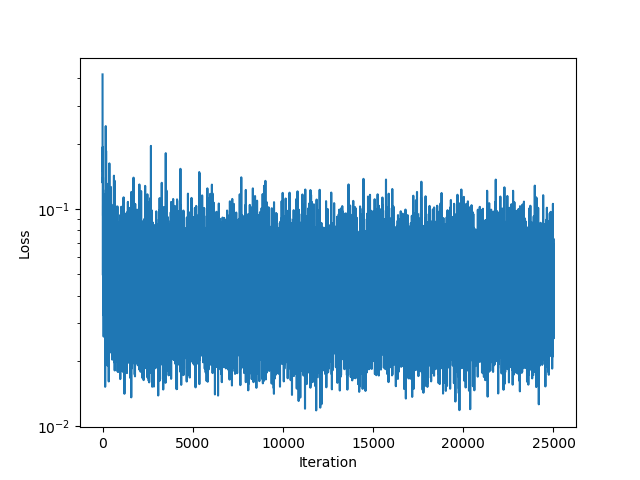
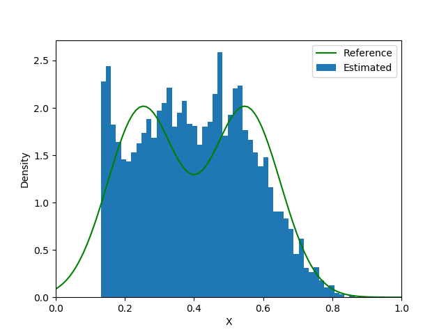
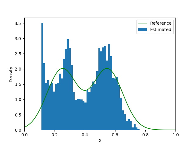
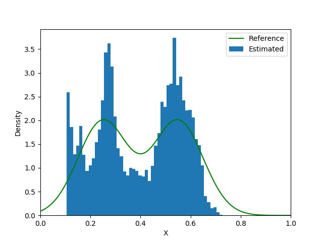
end| Loss Function | Iteration 5000 | Iteration 15000 | Iteration 25000 |
|---|---|---|---|
 |  |  |  |