PDE/ODE Solvers

Runge Kutta Method

The Runge Kutta method is one of the workhorses for solving ODEs. The method is a higher order interpolation to the derivatives. The system of ODE has the form

\[\frac{dy}{dt} = f(y, t, \theta)\]

where $t$ denotes time, $y$ denotes states and $\theta$ denotes parameters.

The Runge-Kutta method is defined as

\[\begin{aligned} k_1 &= \Delta t f(t_n, y_n, \theta)\\ k_2 &= \Delta t f(t_n+\Delta t/2, y_n + k_1/2, \theta)\\ k_3 &= \Delta t f(t_n+\Delta t/2, y_n + k_2/2, \theta)\\ k_4 &= \Delta t f(t_n+\Delta t, y_n + k_3, \theta)\\ y_{n+1} &= y_n + \frac{k_1}{6} +\frac{k_2}{3} +\frac{k_3}{3} +\frac{k_4}{6} \end{aligned}\]

ADCME provides a built-in Runge Kutta solver rk4 and ode45. Consider an example: the Lorentz equation

\[\begin{aligned} \frac{dx}{dt} &= 10(y-x)\\ \frac{dy}{dt} &= x(27-z)-y\\ \frac{dz}{dt} &= xy -\frac{8}{3}z \end{aligned}\]

Let the initial condition be $x_0 = [1,0,0]$, the following code snippets solves the Lorentz equation with ADCME

function f(t, y, θ)
    [10*(y[2]-y[1]);y[1]*(27-y[3])-y[2];y[1]*y[2]-8/3*y[3]]
end
x0 = [1.;0.;0.]
rk4(f, 30.0, 10000, x0)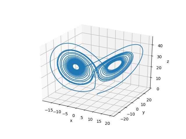

We can also solve three body problem with the Runge-Kutta method. The full script is

# 
# adapted from 
# https://github.com/pjpmarques/Julia-Modeling-the-World/
# 
using Revise
using ADCME
using PyPlot
using Printf

function f(t, y, θ)
    # Extract the position and velocity vectors from the g array
    r0, v0 = y[1:2], y[3:4]
    r1, v1 = y[5:6], y[7:8]
    r2, v2 = y[9:10], y[11:12]
    
    # The derivatives of the position are simply the velocities
    dr0 = v0
    dr1 = v1
    dr2 = v2
    
    # Now calculate the the derivatives of the velocities, which are the accelarations
    # Start by calculating the distance vectors between the bodies (assumes m0, m1 and m2 are global variables)
    # Slightly rewriten the expressions dv0, dv1 and dv2 comprared to the normal equations so we can reuse d0, d1 and d2
    d0  = (r2 - r1) / ( norm(r2 - r1)^3.0 )
    d1  = (r0 - r2) / ( norm(r0 - r2)^3.0 )
    d2  = (r1 - r0) / ( norm(r1 - r0)^3.0 )    
    
    dv0 = m1*d2 - m2*d1
    dv1 = m2*d0 - m0*d2
    dv2 = m0*d1 - m1*d0
    
    # Reconstruct the derivative vector
    [dr0; dv0; dr1; dv1; dr2; dv2]
end

function plot_trajectory(t1, t2)

    t1i = round(Int,NT * t1/T) + 1
    t2i = round(Int,NT * t2/T) + 1
    
    # Plot the initial and final positions
    # In these vectors, the first coordinate will be X and the second Y
    X = 1
    Y = 2
    
    # figure(figsize=(6,6))
    plot(r0[t1i,X], r0[t1i,Y], "ro")
    plot(r0[t2i,X], r0[t2i,Y], "rs")
    plot(r1[t1i,X], r1[t1i,Y], "go")
    plot(r1[t2i,X], r1[t2i,Y], "gs")
    plot(r2[t1i,X], r2[t1i,Y], "bo")
    plot(r2[t2i,X], r2[t2i,Y], "bs")
    
    # Plot the trajectories
    plot(r0[t1i:t2i,X], r0[t1i:t2i,Y], "r-")
    plot(r1[t1i:t2i,X], r1[t1i:t2i,Y], "g-")
    plot(r2[t1i:t2i,X], r2[t1i:t2i,Y], "b-")
    
    # Plot cente of mass
    # plot(cx[t1i:t2i], cy[t1i:t2i], "kx")
    
    # Setup the axis and titles
    xmin = minimum([r0[t1i:t2i,X]; r1[t1i:t2i,X]; r2[t1i:t2i,X]]) * 1.10
    xmax = maximum([r0[t1i:t2i,X]; r1[t1i:t2i,X]; r2[t1i:t2i,X]]) * 1.10
    ymin = minimum([r0[t1i:t2i,Y]; r1[t1i:t2i,Y]; r2[t1i:t2i,Y]]) * 1.10
    ymax = maximum([r0[t1i:t2i,Y]; r1[t1i:t2i,Y]; r2[t1i:t2i,Y]]) * 1.10
    
    axis([xmin, xmax, ymin, ymax])
    title(@sprintf "3-body simulation for t=[%.1f .. %.1f]" t1 t2)
end;

m0 = 5.0
m1 = 4.0
m2 = 3.0

# Initial positions and velocities of each body (x0, y0, vx0, vy0) 
gi0 = [ 1.0; -1.0; 0.0; 0.0]
gi1 = [ 1.0;  3.0; 0.0; 0.0]
gi2 = [-2.0; -1.0; 0.0; 0.0]


T  = 30.0
NT  = 500*300
g0  = [gi0; gi1; gi2]

res_ = ode45(f, T, NT, g0)

sess = Session(); init(sess)
res = run(sess, res_)

r0, v0, r1, v1, r2, v2 = res[:,1:2], res[:,3:4], res[:,5:6], res[:,7:8], res[:,9:10], res[:,11:12]

figure(figsize=[4,1])
subplot(131); plot_trajectory(0.0,10.0)
subplot(132); plot_trajectory(10.0,20.0)
subplot(133); plot_trajectory(20.0,30.0)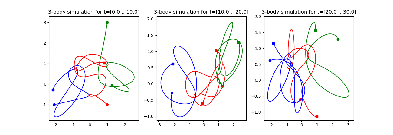

Explicit Newmark Scheme

ExplicitNewmark provides an explicit Newmark integrator for

\[M \ddot{\mathbf{d}} + Z_1 \dot{\mathbf{d}} + Z_2 \mathbf{d} + f = 0\]

The numerical scheme is given by

\[\left(\frac{1}{\Delta t^2} M + \frac{1}{2\Delta t}Z_1\right)d^{n+1} = \left(\frac{2}{\Delta t^2} M - \frac{1}{2\Delta t}Z_2\right)d^n - \left(\frac{1}{\Delta t^2} M - \frac{1}{2\Delta t}Z_1\right) d^{n-1} - f^n\]

We consider an example:

\[\mathbf{d} = \begin{bmatrix}e^{-t}\\ e^{-2t}\end{bmatrix}\]

and

\[M = \begin{bmatrix}1 & 2\\3 &4 \end{bmatrix}\qquad Z_1 = \begin{bmatrix}5 & 6\\7 &8 \end{bmatrix}\qquad Z_2 =\begin{bmatrix}9 & 10\\11 &12 \end{bmatrix} $$ The function $f$ is given by $$f(t) = -\begin{bmatrix}5e^{-t} + 6e^{-2t}\\ 7 e^{-t} + 12 e^{-2t}\end{bmatrix}\]

We can carry out the simulation using the following codes:

using ADCME 
using PyPlot 

M = Float64[1 2;3 4]
Z1 = Float64[5 6;7 8]
Z2 = Float64[9 10;11 12]

NT = 200
Δt = 1/NT 

F = zeros(NT+1, 2)
for i = 1:NT+1
    t = (i-1)*Δt 
    F[i,1] = -(5exp(-t) + 6exp(-2t))
    F[i,2] = -(7exp(-t) + 12exp(-2t))
end 
F = constant(F)

en = ExplicitNewmark(M, Z1, Z2, Δt)

function condition(i, d)
    i<=NT
end

function body(i, d)
    d0 = read(d, i-1)
    d1 = read(d, i)
    d2 = step(en, d0, d1, F[i-1])
    i+1, write(d, i+1, d2)
end

d = TensorArray(NT+1)
d = write(d, 1, [1.0;1.0])
d = write(d, 2, [exp(-Δt);exp(-2Δt)])
i = constant(2, dtype = Int32)
_, d = while_loop(condition, body, [i, d])
d = stack(d)

sess = Session(); init(sess)
D = run(sess, d)
ts = (0:NT)*Δt
close("all")
plot(ts, D[:, 1], "b.")
plot(ts, D[:,2], "g.")
plot(ts, exp.(-ts), "r--")
plot(ts, exp.(-2ts), "r--")
xlabel("t"); ylabel("y")
savefig("ode_solution.png")

Build Your Own Solvers

Sometimes it is helpful to build your own ODE/PDE solvers. The basic routine is

Implement the one step state transition function;
Use while_loop to build the time integrator.

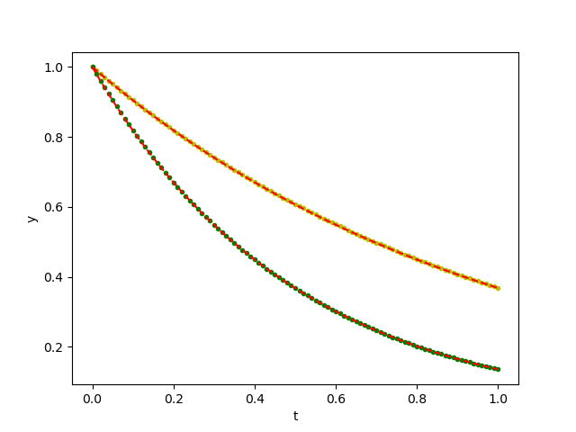
As an example, we build a second-order Runge-Kutta scheme for

\[\dot{\mathbf{d}} + \beta \mathbf{d} = \mathbf{t}\]

The numerical scheme is

\[\begin{aligned}h_1 &= -\beta \mathbf{d}^n + \mathbf{t}^n\\ h_2 &= -\beta(\mathbf{d}^n + \Delta t h_1) + \mathbf{t}^n\\ \mathbf{d}^{n+1} &= \mathbf{d}^n + \frac{\Delta t}{2}(h_1 + h_2)\end{aligned}\]

The state transition function has the following form

function rk_one_step(d2, t)
    h1 = -β*d2 + t 
    h2 = -β*(d2+Δt*h1)+t 
    d2 + Δt/2*(h1+h2)
end

Now consider an analytical solution

\[\mathbf{d} = \begin{bmatrix}e^{-t}\\e^{-2t}\end{bmatrix}, \quad \beta = 2\]

Then we have

\[\mathbf{t} = \begin{bmatrix}e^{-t}\\0\end{bmatrix}\]

The main code is as follows

using ADCME
using PyPlot

NT = 100
Δt = 1/NT 
ts = Array((0:NT)*Δt)
t = constant([exp.(-ts) zeros(NT+1)])
β = 2.0



function condition(i, d)
    i<=NT
end

function body(i, d)
    d0 = read(d, i)
    d1 = rk_one_step(d0, t[i])
    i+1, write(d, i+1, d1) 
end

d = TensorArray(NT+1)
d = write(d, 1, ones(2))
i = constant(1, dtype = Int32)
_, d = while_loop(condition, body, [i, d])
d = stack(d)

sess = Session(); init(sess)
D = run(sess, d)

close("all")
plot(ts, D[:,1], "y.")
plot(ts, D[:,2], "g.")
plot(ts, exp.(-ts), "r--")
plot(ts, exp.(-2ts), "r--")
xlabel("t"); ylabel("y")
savefig("ode_solution2.png")