Bayesian Neural Networks

Motivation

Bayesian neural networks are different from plain neural networks in that weights and biases in Bayesian neural networks are interpreted in a probabilistic manner. Instead of finding a point estimation of weights and biases, in Bayesian neural networks, a prior distribution is assigned to the weights and biases, and a posterior distribution is obtained from the data. It relies on the Bayes formula

Here $\mathcal{D}$ is the data, e.g., the input-output pairs of the neural network $\{(x_i, y_i)\}$, $w$ is the weights and biases of the neural network, and $p(w)$ is the prior distribution.

If we have a full posterior distribution $p(w|\mathcal{D})$, we can conduct predictive modeling using

However, computing $p(w|\mathcal{D})$ is usually intractable since we need to compute the normalized factor $p(\mathcal{D}) = \int p(\mathcal{D}|w)p(w) dw$, which requires us to integrate over all possible $w$. Traditionally, Markov chain Monte Carlo (MCMC) has been used to sample from $p(w|\mathcal{D})$ without evaluating $p(\mathcal{D})$. However, MCMC can converge very slowly and requires a voluminous number of sampling, which can be quite expensive.

Variational Inference

In Bayesian neural networks, the idea is to approximate $p(w|\mathcal{D})$ using a parametrized family $p(w|\theta)$, where $\theta$ is the parameters. This method is called variational inference. We minimize the KL divergeence between the true posterior and the approximate posterial to find the optimal $\theta$

Evaluating $p(\mathcal{D})\geq 0$ is intractable, so we seek to minimize a lower bound of the KL divergence, which is known as variational free energy

In practice, thee variational free energy is approximated by the discrete samples

Parametric Family

In Baysian neural networks, the parametric family is usually chosen to be the Gaussian distribution. For the sake of automatic differentiation, we usually parametrize $w$ using

Here $\theta = (\mu, \sigma)$. The prior distributions for $\mu$ and $\sigma$ are given as hyperparameters. For example, we can use a mixture of Gaussians as prior

The advantage of Equation 1 is that we can easily obtain the log probability $\log p(w|\theta)$.

Because $\sigma$ should always be positive, we can instead parametrize another parameter $\rho$ and transform $\rho$ to $\sigma$ using a softplus function

Example

Now let us consider a concrete example. The following example is adapted from this post.

Generating Training Data

We first generate some 1D training data

using ADCME
using PyPlot 
using ProgressMeter
using Statistics

function f(x, σ)
    ε = randn(size(x)...) * σ
    return 10 * sin.(2π*x) + ε
end

batch_size = 32
noise = 1.0

X = reshape(LinRange(-0.5, 0.5, batch_size)|>Array, :, 1)
y = f(X, noise)
y_true = f(X, 0.0)

close("all")
scatter(X, y, marker="+", label="Training Data")
plot(X, y_true, label="Truth")
legend()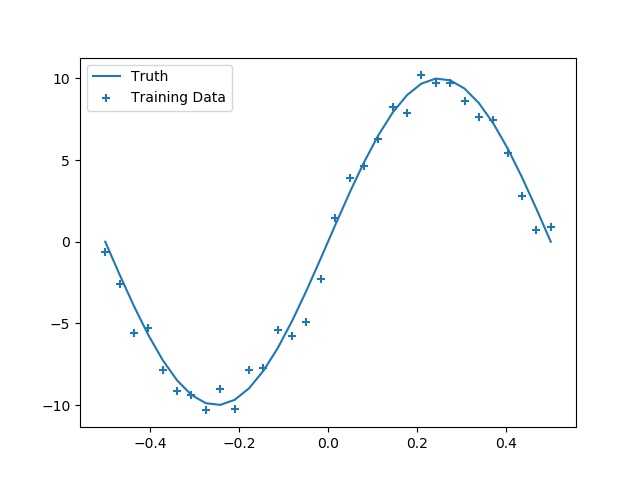

Construct Bayesian Neural Network

mutable struct VariationalLayer
    units
    activation
    prior_σ1
    prior_σ2
    prior_π1
    prior_π2
    Wμ
    bμ
    Wρ
    bρ
    init_σ
end

function VariationalLayer(units; activation=relu, prior_σ1=1.5, prior_σ2=0.1,
        prior_π1=0.5)
    init_σ = sqrt(
        prior_π1 * prior_σ1^2 + (1-prior_π1)*prior_σ2^2
    )
    VariationalLayer(units, activation, prior_σ1, prior_σ2, prior_π1, 1-prior_π1,
                        missing, missing, missing, missing, init_σ)
end

function kl_loss(vl, w, μ, σ)
    dist = ADCME.Normal(μ,σ)
    return sum(logpdf(dist, w)-logprior(vl, w))
end

function logprior(vl, w)
    dist1 = ADCME.Normal(constant(0.0), vl.prior_σ1)
    dist2 = ADCME.Normal(constant(0.0), vl.prior_σ2)
    log(vl.prior_π1*exp(logpdf(dist1, w)) + vl.prior_π2*exp(logpdf(dist2, w)))
end

function (vl::VariationalLayer)(x)
    x = constant(x)
    if ismissing(vl.bμ)
        vl.Wμ = get_variable(vl.init_σ*randn(size(x,2), vl.units))
        vl.Wρ = get_variable(zeros(size(x,2), vl.units))
        vl.bμ = get_variable(vl.init_σ*randn(1, vl.units))
        vl.bρ = get_variable(zeros(1, vl.units))
    end
    Wσ = softplus(vl.Wρ)
    W = vl.Wμ + Wσ.*normal(size(vl.Wμ)...) 
    bσ = softplus(vl.bρ)
    b = vl.bμ + bσ.*normal(size(vl.bμ)...)
    loss = kl_loss(vl, W, vl.Wμ, Wσ) + kl_loss(vl, b, vl.bμ, bσ)
    out = vl.activation(x * W + b)
    return out, loss 
end

function neg_log_likelihood(y_obs, y_pred, σ)
    y_obs = constant(y_obs)
    dist = ADCME.Normal(y_pred, σ)
    sum(-logpdf(dist, y_obs))
end

ipt = placeholder(X)
x, loss1 = VariationalLayer(20, activation=relu)(ipt)
x, loss2 = VariationalLayer(20, activation=relu)(x)
x, loss3 = VariationalLayer(1, activation=x->x)(x)

loss_lf = neg_log_likelihood(y, x, noise)
loss = loss1 + loss2 + loss3 + loss_lf

Optimization

We use an ADAM optimizer to optimize the loss function. In this case, quasi-Newton methods that are typically used for deterministic function optimization are not appropriate because the loss function essentially involves stochasticity.

Another caveat is that because the neural network may have many local minimum, we need to run the optimizer multiple times in order to obtain a good local minimum.

opt = AdamOptimizer(0.08).minimize(loss)
sess = Session(); init(sess)
@showprogress for i = 1:5000
    run(sess, opt)
end


X_test = reshape(LinRange(-1.5,1.5,32)|>Array, :, 1)
y_pred_list = []
@showprogress for i = 1:10000
    y_pred = run(sess, x, ipt=>X_test)
    push!(y_pred_list, y_pred)
end

y_preds = hcat(y_pred_list...)

y_mean = mean(y_preds, dims=2)[:]
y_std = std(y_preds, dims=2)[:]

close("all")
plot(X_test, y_mean)
scatter(X[:], y[:], marker="+")
fill_between(X_test[:], y_mean-2y_std, y_mean+2y_std, alpha=0.5)