Distributed Scientific Machine Learning using MPI
Many large-scale scientific computing involves parallel computing. Among many parallel computing models, the MPI is one of the most popular models. In this section, we describe how ADCME can work with MPI for solving inverse modeling. Specifically, we describe how gradients can be back-propagated via MPI function calls.
Message Passing Interface (MPI) is an interface for parallel computing based on message passing models. In the message passing model, a master process assigns work to workers by passing them a message that describes the work. The message may be data or meta information (e.g., operations to perform). A consensus was reached around 1992 and the MPI standard was born. MPI is a definition of interface, and the implementations are left to hardware venders.
MPI Support in ADCME
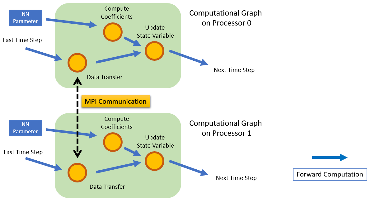
The ADCME solution to distributed computing for scientific machine learning is to provide a set of "data communication" nodes in the computational graph. Each machine (MPI processor) runs an identical computational graph. The computational nodes are executed independently on each processor, and the data communication nodes need to synchronize among different processors.
These data communication nodes are implemented using MPI APIs. They are not necessarily blocking operations, but because ADCME respects the data dependency of computation, they act like blocking operations and the child operators are executed only when data communication is finished. For example, in the following example,
b = mpi_op(a)
c = custom_op(b)
even though mpi_op and custom_op can overlap, ADCME still sequentially execute these two operations.
This blocking behavior simplifies the synchronization logic as well as the implementation of gradient back-propagation while harming little performance.

ADCME provides a set of commonly used MPI operators. See MPI Operators. Basically, they are
mpi_init,mpi_finalize: Initialize and finalize MPI session.mpi_rank,mpi_size: Get the MPI rank and size.mpi_sum,mpi_bcast: Sum and broadcast tensors in different processors.mpi_send,mpi_recv: Send and receive operators.
The above two set of operators support automatic differentiation. They were implemented with MPI adjoint methods, which have existed in academia for decades.
This section shows how to configure MPI for distributed computing in ADCME.
Limitations
Despite that the provided mpi_* operations meet most needs, some sophisticated data communication operations may not be easily expressed using these APIs. For example, when solving the Poisson's equation on a uniform grid, we may decompose the domain into many squares, and two adjacent squares exchange data in each iteration. A sequence of mpi_send, mpi_recv will likely cause deadlock.
Just like when it is difficult to use automatic differentiation to implement a forward computation and its gradient back-propagation, we resort to custom operators, it is the same case for MPI. We can design a specialized custom operator for data communication. To resolve the deadlock problem, we found the asynchronous sending, followed by asynchronous receiving, and then followed by waiting, a very general and convenient way to implement custom operators.

Another limitation for ADCME is that currently, for performance, we need to set the total number of threads per MPI process to be 1
config = tf.ConfigProto(inter_op_parallelism_threads=1)
sess = Session(config = config)
Otherwise, there will be significant cost for synchronization between different threads for the MPI operation kernel. Setting inter_op_parallelism_threads=1 limits ADCME to execute one kernel at a time, although each kernel can still utilize multiple threads. One solution is to use a specialized executed policy for MPI kernels–-they should always executed by one thread. Nevertheless, the optimal policy is application dependent and the current model fits a broad range of applications.
Implementing Custom Operators using MPI
We can also make custom operators with MPI. Let us consider computing
Each $f_i$ is a very expensive function so it makes sense to use MPI to split the jobs on different processors. To simplify the problem, we consider
where $f_i(\theta) = \theta^{i-1}$.

Using the ADCME MPI API, we have the following code (test_simple.jl)
using ADCME

mpi_init()
θ = placeholder(ones(1))
fθ = mpi_bcast(θ)
l = fθ^mpi_rank()
L = sum(mpi_sum(l))
g = gradients(L, θ)
sess = Session(); init(sess)
L_ = run(sess, L, θ=>ones(1)*2.0)
g_ = run(sess, g, θ=>ones(1)*2.0)

if mpi_rank()==0
    @info  L_, g_
end
mpi_finalize()
We run the program with 4 processors
mpirun -n 4 julia test_simple.jlWe have the results:
[ Info: (15.0, [17.0])Optimization
For solving inverse problems using distributed computing, an MPI-capable optimizer is required. The ADCME solution to distributed optimization is that the master machine holds, distributes and updates the optimizable variables. The gradients are calculated in the same device where the corresponding forward computation is done. Therefore, for a given serial optimizer, we can refactor it to a distributed one by letting worker nodes wait for instructions from the master node to compute either the objective function or the gradient.
This idea is implemented in the ADOPT.jl package, a customized version of Optim.jl.

In the following, we try to solve
using MPI-enabled LBFGS optimizer.
using ADCME
using ADOPT
mpi_init()
θ = placeholder(ones(1))
fθ = mpi_bcast(θ)
l = fθ^mpi_rank()
L = (sum(mpi_sum(l)) - 2.0)^2
sess = Session(); init(sess)

f = x->run(sess, L, θ=>x)
g! = (G, x)->(G[:] = run(sess, g, θ=>x))

options = Options()
if mpi_rank()==0
    options.show_trace = true
end
mpi_optimize(f, g!, ones(1), ADOPT.LBFGS(), options)
if mpi_rank()==0
    @info  result.minimizer, result.minimum
end

mpi_finalize()
The expected output is
Iter     Function value   Gradient norm
     0     4.000000e+00     2.400000e+01
 * time: 0.00012421607971191406
     1     6.660012e-01     7.040518e+00
 * time: 1.128843069076538
     2     7.050686e-02     1.322515e+00
 * time: 1.210536003112793
     3     2.254820e-03     2.744374e-01
 * time: 1.2910940647125244
     4     4.319834e-07     3.908046e-03
 * time: 1.3442070484161377
     5     2.894433e-16     1.011994e-07
 * time: 1.3975300788879395
     6     0.000000e+00     0.000000e+00
 * time: 1.4507441520690918
[ Info: ([0.5436890126920764], 0.0)
Reduce Sum
using ADCME

mpi_init()
r = mpi_rank()
a = constant(Float64.(Array(1:10) * r))
b = mpi_sum(a)

L = sum(b)
g = gradients(L, a)
sess = Session(); init(sess)
v, G = run(sess, [b,g])
mpi_finalize()
Broadcast
using ADCME

mpi_init()
r = mpi_rank()
a = constant(ones(10) * r)
b = mpi_bcast(a, 3)
L = sum(b^2)
L = mpi_sum(L)
g = gradients(L, a)

sess = Session(); init(sess)
v, G = run(sess, [b, G])
mpi_finalize()
Send and Receive
# mpiexec.exe -n 4 julia .\mpisum.jl
using ADCME

mpi_init()
r = mpi_rank()
a = constant(ones(10) * r)
a = mpi_sendrecv(a, 0, 2)

L = sum(a^2)
g = gradients(L, a)

sess = Session(); init(sess)
v, G = run(sess, [a,g])
mpi_finalize()
mpi_sendrecv is a lightweight wrapper for mpi_send followed by mpi_recv. Equivalently, we have
if r==2
    global a
    a = mpi_send(a, 0)
end
if r==0
    global a
    a = mpi_recv(a,2)
end
Solving the Heat Equation
In this section, we consider solving the Poisson equation
We discretize the above PDE with an explicit finite difference scheme
To mitigate the computational and memory requirement, we use MPI APIs to implement a domain decomposition solver for the heat equation. The mesh is divided into $N\times M$ rectangle patches. We implemented two operation:
heat_op, which updates $u_{ij}^{n+1}$ using Equation 1 for a specific patch, with state variables $u_{ij}^n$ in the current rectangle patch and on the boundary (from adjacent patches).data_exchange, which is a data communication operator that sends the boundary data to adjacent patches and receives boundary data from other patches.

Then the time marching scheme can be implemented with the following code:
function heat_update_u(u, kv, f)
    r = mpi_rank()
    I = div(r, M)
    J = r%M

    up_ = constant(zeros(m))
    down_ = constant(zeros(m))
    left_ = constant(zeros(n))
    right_ = constant(zeros(n))


    up = constant(zeros(m))
    down = constant(zeros(m))
    left = constant(zeros(n))
    right = constant(zeros(n))

    (I>0) && (up = u[1,:])
    (I<N-1) && (down = u[end,:])
    (J>0) && (left = u[:,1])
    (J<M-1) && (right = u[:,end])

    left_, right_, up_, down_ = data_exchange(left, right, up, down)

    u = heat(u, kv, up_, down_, left_, right_, f, h, Δt)
end
An MPI-capable heat equation time integrator can be implemented with
function heat_solver(u0, kv, f, NT=10)
    f = constant(f)
    function condition(i, u_arr)
        i<=NT
    end
    function body(i, u_arr)
        u = read(u_arr, i)
        u_new = heat_update_u(u, kv, f[i])
        # op = tf.print(r, i)
        # u_new = bind(u_new, op)
        i+1, write(u_arr, i+1, u_new)
    end
    i = constant(1, dtype =Int32)
    u_arr = TensorArray(NT+1)
    u_arr = write(u_arr, 1, u0)
    _, u = while_loop(condition, body, [i, u_arr])
    reshape(stack(u), (NT+1, n, m))
end
For example, we can implement the heat solver with diffusivity coefficient $K_0$ and initial condition $u_0$ with the following code:
K = placeholder(K0)
a_ = mpi_bcast(K)
sol = heat_solver(u0, K_, F, NT)