Coupled Viscoelasticity and Single Phase Flow
We have considered inverse modeling for viscoelasticity and coupled elasticity and single phase flow inversion. A more complex case is when the constitutive relation is given by the viscoelasticity and the dynamics is governed by the coupled viscoelasticity and single phase flow equation. We consider the same governing equation as the poreelasticity
\[\begin{aligned} \mathrm{div}\sigma(u) - b \nabla p &= 0\\ \frac{1}{M} \frac{\partial p}{\partial t} + b\frac{\partial \varepsilon_v(u)}{\partial t} - \nabla\cdot\left(\frac{k}{B_f\mu}\nabla p\right) &= f(x,t) \end{aligned}\]
with boundary conditions
\[\begin{aligned} \sigma n = 0,\quad x\in \Gamma_{N}^u, \qquad u=0, \quad x\in \Gamma_D^u\\ -\frac{k}{B_f\mu}\frac{\partial p}{\partial n} = 0,\quad x\in \Gamma_{N}^p, \qquad p=g, \quad x\in \Gamma_D^p \end{aligned}\]
and the initial condition
\[p(x,0) = 0,\ u(x,0) =0,\ x\in \Omega\]
The only difference is that the consitutive relation is given by the Maxwell material equation, which has the following form in the discretization (for the definition of $H$ and $S$, see here)
\[\sigma^{n+1} = H \varepsilon^{n+1} + S \sigma^n - H\varepsilon^n\]
Then the discretization for the mechanics is
\[\int_\Omega H \varepsilon^{n+1} : \delta \varepsilon \;\mathrm{d}x- \int_\Omega b p \delta u \;\mathrm{d}x = \int_{\partial \Omega} \mathbf{t}\delta u \;\mathrm{d}s + \int_{\Omega} H\varepsilon^n : \delta\varepsilon \;\mathrm{d} x - \int_\Omega S\sigma^n : \delta \varepsilon \;\mathrm{d} x\]
For the discretization of the fluid equation, see here.
Forward Simulation
To have an overview of the viscoelasticiy, we conduct the forward simulation in the injection-production model. An injection well is located on the left while a production well is located on the right. We impose the Dirichlet boundary conditions for $u$ and no flow boundary conditions for the pressure on four sides. We run the results with Lamé constants $\lambda=2.0$ and $\mu=0.5$, and three different viscosity $\eta = 10000, 1$, and $0.1$. The case $\eta = 10000$ corresponds to a nearly linear elastic constitutive relation. The typical characteristics of viscoelasticity in our experiments are that they usually possess larger stresses and smaller displacements.
| Description | $\eta=10000$ | $\eta=1$ | $\eta=0.1$ |
|---|---|---|---|
| Pressure |  |  |  |
| $\sigma_{xx}$ |  |  |  |
| $\sigma_{xy}$ |  |  |  |
| $\sigma_{yy}$ |  |  |  |
| $u$ |  |  |  |
| $v$ |  |  |  |
| $\sigma_{xx}$ at the center point | 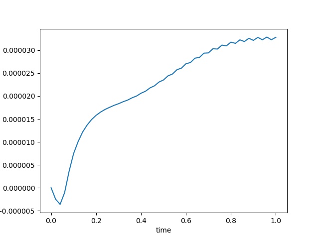 | 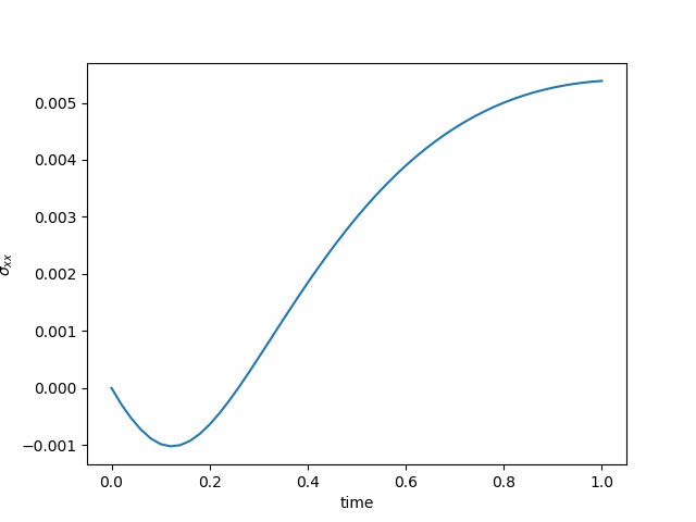 | 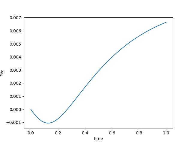 |
| $u$ at the center point | 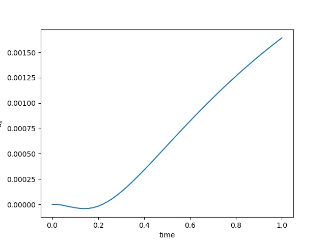 | 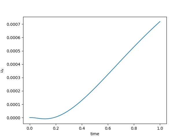 | 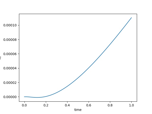 |
| $\varepsilon_{xx}$ at the center point | 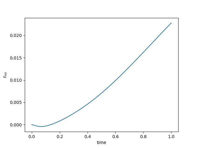 | 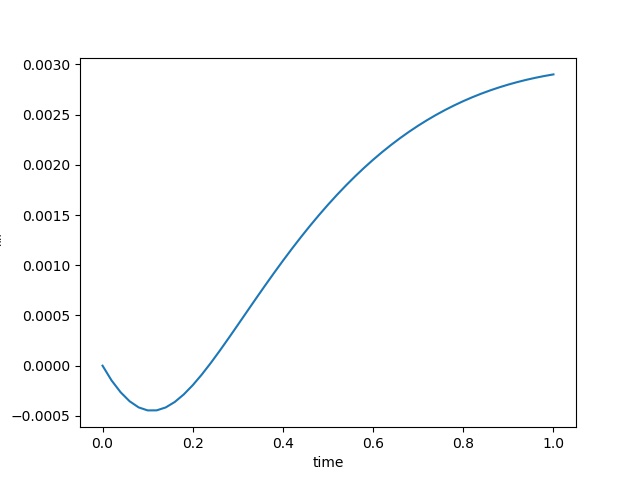 |  |
Inverse Modeling
In the inverse modeling, the initial conditions and boundary conditions are
Here $u$, $\sigma$, and $p$ are all initialized to zero.
Fixed Dirichlet boundaries for $u$ on the bottom.
Traction-free boundary conditions (free surface) for $u$ on the other three sides
No-flow condition for $p$ on all sides.
We have 5 sets of training data, each corresponds to a Delta production (injection) source with the magnitude $0.2i$, $i=1,2,3,4$ and 5. We show a typical dataset below.
| Pressure | $\sigma_{xx}$ | $\sigma_{yy}$ | $\sigma_{xy}$ | $u$ | $v$ |
|---|---|---|---|---|---|
 |  |  |  |  |  |
| Displacement | $\sigma_{xx}$ at the center point | $\varepsilon_{xx}$ at the center point | $u$ at the center point |
|---|---|---|---|
 |  |  |  |
The observation data is the $x$-direction displacement at all time steps on the surface. We will consider several kinds of inversion.
Parametric inversion. In this case, we assume we already know the form of the consitutitve relation and we only need to estimate $\mu$, $\lambda$ and $\eta$. code
Linear elasticity approximation. In this case, the constitutive relation is assumed to have the linear elasticity form code
\[\sigma = H\varepsilon\]
Here $H$ is an unknown SPD matrix.
Direct inversion. The constitutive relation is substituted by
$\sigma^{n+1} = \mathcal{NN}(\sigma^n, \varepsilon^n)$
where $\mathcal{NN}$ is a neural network. code
Implicit inversion. The constitutive relation is subsituted by
$\sigma^{n+1} = \mathcal{NN}(\sigma^n, \varepsilon^n) + H\varepsilon^{n+1}$
where $\mathcal{NN}$ is a neural network and $H$ is an unknown SPD matrix. The motivation of this form is to improve the conditioning of the implicit numerical scheme. code
To evaluate the inverse modeling result, we consider a test dataset which corresponds to the magnitude 0.5 for the Delta sources. We measure the displacement and Von Mises stress. For the first inversion, we report the values.
For the parametric inversion, we have the following result
 |  |  |
|---|---|---|
| Loss Function | Von Mises Stress | Displacement |
| Parameter | Initial Guess | Estimated | True |
|---|---|---|---|
| $\mu$ | 1.5 | 0.49999986292871396 | 0.5 |
| $\lambda$ | 1.5 | 1.9999997784851993 | 2.0 |
| $\eta$ | 1.5 | 0.9999969780184615 | 1.0 |
For the other three types of inversion, the results are presented below
| Reference | Linear Elasticity | Direct | Implicit |
|---|---|---|---|
 |  |  |  |
 |  |  |  |
The results are reported at 2000-th iteration. In terms of the Von Mises stress, we see that the direct training gives us the best result (note the scale of the colorbar).
Forward Simulation Codes
using Revise
using AdFem
using PyCall
using LinearAlgebra
using ADCME
using MAT
using PyPlot
np = pyimport("numpy")

# Domain information
NT = 50
Δt = 1/NT
n = 20
m = 2*n
h = 1.0/n
bdnode = Int64[]
for i = 1:m+1
    for j = 1:n+1
        if i==1 || i==m+1 || j==1|| j==n+1
            push!(bdnode, (j-1)*(m+1)+i)
        end
    end
end

is_training = false
b = 1.0

invη = 1.0
if length(ARGS)==1
    global invη = parse(Float64, ARGS[1])
end

λ = constant(2.0)
μ = constant(0.5)
invη = constant(invη)

iS = tensor(
    [1+2/3*μ*Δt*invη -1/3*μ*Δt*invη 0.0
    -1/3*μ*Δt*invη 1+2/3*μ*Δt*invη 0.0
    0.0 0.0 1+μ*Δt*invη]
)
S = inv(iS)
H = S * tensor([
    2μ+λ λ 0.0
    λ 2μ+λ 0.0
    0.0 0.0 μ
])


Q = SparseTensor(compute_fvm_tpfa_matrix(m, n, h))
K = compute_fem_stiffness_matrix(H, m, n, h)
L = SparseTensor(compute_interaction_matrix(m, n, h))
M = SparseTensor(compute_fvm_mass_matrix(m, n, h))
A = [K -b*L'
b*L/Δt 1/Δt*M-Q]
A, Abd = fem_impose_coupled_Dirichlet_boundary_condition(A, bdnode, m, n, h)
# error()
U = zeros(m*n+2(m+1)*(n+1), NT+1)
x = Float64[]; y = Float64[]
for j = 1:n+1
    for i = 1:m+1
        push!(x, (i-1)*h)
        push!(y, (j-1)*h)
    end
end

injection = (div(n,2)-1)*m + 3
production = (div(n,2)-1)*m + m-3


function condition(i, tas...)
    i<=NT
end

function body(i, tas...)
    ta_u, ta_ε, ta_σ = tas
    u = read(ta_u, i)
    σ0 = read(ta_σ, i)
    ε0 = read(ta_ε, i)
    rhs1 = compute_fem_viscoelasticity_strain_energy_term(ε0, σ0, S, H, m, n, h)
    rhs2 = zeros(m*n)
    rhs2[injection] += 1.0
    rhs2[production] -= 1.0
    rhs2 += b*L*u[1:2(m+1)*(n+1)]/Δt +
            M * u[2(m+1)*(n+1)+1:end]/Δt
    rhs = [rhs1;rhs2]
    o = A\rhs

    ε = eval_strain_on_gauss_pts(o, m, n, h)
    σ = σ0*S + (ε - ε0)*H
    ta_u = write(ta_u, i+1, o)
    ta_ε = write(ta_ε, i+1, ε)
    ta_σ = write(ta_σ, i+1, σ)
    i+1, ta_u, ta_ε, ta_σ
end

i = constant(1, dtype=Int32)
ta_u = TensorArray(NT+1); ta_u = write(ta_u, 1, constant(zeros(2(m+1)*(n+1)+m*n)))
ta_ε = TensorArray(NT+1); ta_ε = write(ta_ε, 1, constant(zeros(4*m*n, 3)))
ta_σ = TensorArray(NT+1); ta_σ = write(ta_σ, 1, constant(zeros(4*m*n, 3)))
_, u_out, ε_out, σ_out = while_loop(condition, body, [i, ta_u, ta_ε, ta_σ])
u_out = stack(u_out)
u_out.set_shape((NT+1, size(u_out,2)))
σ_out = stack(σ_out)
ε_out = stack(ε_out)

upper_idx = Int64[]
for i = 1:m+1
    push!(upper_idx, (div(n,3)-1)*(m+1)+i)
    push!(upper_idx, (div(n,3)-1)*(m+1)+i + (m+1)*(n+1))
end
for i = 1:m
    push!(upper_idx, (div(n,3)-1)*m+i+2(m+1)*(n+1))
end

sess = Session(); init(sess)
U, Sigma, Varepsilon, ev = run(sess, [u_out,σ_out,ε_out, invη])
visualize_displacement(U'|>Array, m, n, h, name="_visco$ev")
visualize_pressure(U'|>Array, m, n, h, name="_visco$ev")
visualize_displacement(U'|>Array, m, n, h, name="_visco$ev")
visualize_stress(Sigma[:,:,1]'|>Array, m, n, h, name="xx_visco$ev")
visualize_stress(Sigma[:,:,2]'|>Array, m, n, h, name="yy_visco$ev")
visualize_stress(Sigma[:,:,3]'|>Array, m, n, h, name="xy_visco$ev")


idx = m÷2 + (n÷2)*m
close("all")
plot(LinRange(0,1.0, NT+1),Sigma[:,4*(idx-1)+1,1])
xlabel("time")
ylabel("\$\\sigma_{xx}\$")
savefig("sigmaxx$ev.jpeg")

close("all")
plot(LinRange(0,1.0, NT+1),Varepsilon[:,4*(idx-1)+1,1])
xlabel("time")
ylabel("\$\\varepsilon_{xx}\$")
savefig("varepsilonxx$ev.jpeg")

idx = m÷2 + (n÷2)*(m+1)
close("all")
plot(LinRange(0,1.0, NT+1),U[:,4*(idx-1)+1])
xlabel("time")
ylabel("\$u_x\$")
savefig("ux$ev.jpeg")