Working with 3D Domains

AdFem also supports finite element analysis in 3D. In this section, we illustrate how to work with 3D domains in AdFem with a simple Poisson's equation example. The governing equation is given by

\[\nabla \cdot (\kappa(x) \nabla u) = - f(x) \text{ in } \Omega, \quad u(x) = 0 \text{ on } \partial \Omega \tag{1}\]

Here the diffusivity coefficient is given by

\[\kappa(x) = \frac{1}{a + \|x\|^2_2}\]

where $a$ is a quantity of interest, which can be the parameter to be calibrated in the inverse problem. For simplicity, we let

\[f(x) = 1\]

The first step is to derive a weak form of Eq. 1, which is given by

\[(\kappa(x) \nabla u, \nabla v) = (f, v), \forall v \in H^1_0(\Omega) \tag{2}\]

We now consider implementing a numerical solver for Eq. 2. I annotated the code in detail for convenience.

using AdFem

# construct a 3D cube domain [0,1]^3, and each dimension is divided into 20 equal length intervals
mmesh = Mesh3(20, 20, 20, 1/20)

# evaluate kappa on the Gauss points
xy = gauss_nodes(mmesh)
a = Variable(0.1)
κ = 1/(a+xy[:,1].^2 + xy[:,2].^2 + xy[:,3].^2)

# construct the coefficient matrix and the right hand side
K = compute_fem_laplace_matrix1(κ, mmesh)
rhs = compute_fem_source_term1(ones(get_ngauss(mmesh)), mmesh)

# impose the boundary condition
bd = bcnode(mmesh)
K, rhs = impose_Dirichlet_boundary_conditions(K, rhs, bd, zeros(length(bd)))

# solve the linear system 
sol = K\rhs
sess = Session(); init(sess)
SOL = run(sess, sol)

We also provide the FEniCS code for solving the same problem

from dolfin import *
import matplotlib.pyplot as plt
import numpy as np

# Create mesh and define function space
mesh = UnitCubeMesh(20,20,20)
V = FunctionSpace(mesh, "Lagrange", 1)

# Define Dirichlet boundary (x = 0 or x = 1)
def boundary(x):
    return x[0] < DOLFIN_EPS or x[0] > 1.0 - DOLFIN_EPS or \
        x[1] < DOLFIN_EPS or x[1] > 1.0 - DOLFIN_EPS or \
        x[2] < DOLFIN_EPS or x[2] > 1.0 - DOLFIN_EPS

# Define boundary condition
u0 = Constant(0.0)
bc = DirichletBC(V, u0, boundary)

# Define variational problem
u = TrialFunction(V)
v = TestFunction(V)
f = Expression("1.0", degree=2)
kappa = Expression("1/(0.1 + x[0]*x[0] + x[1]*x[1] + x[2]*x[2])", degree=2)
a = inner(kappa*grad(u), grad(v))*dx
L = f*v*dx

# Compute solution
u = Function(V)
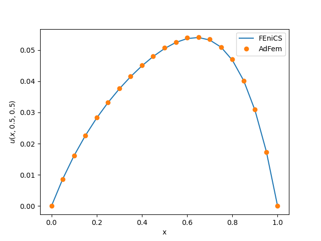
solve(a == L, u, bc)

We compare the AdFem result and FEniCS result for $u(x, 0.5, 0.5)$. We can see that our result is consistent with FEniCS.

Like 2D cases, our numerical solvers are AD-capable. For example, given a loss function

loss = sum(u^2)

We can take the derivative of loss with respect to the quantity of interest a:

gradients(loss, a)

AdFem provides many visualization tools for 3D unstructured mesh. For example, you can try visualize_mesh to visualize mmesh in the code. You can use s/w buttons to toggle between solid and wireframe mode.

Solid Mode	Wireframe Mode

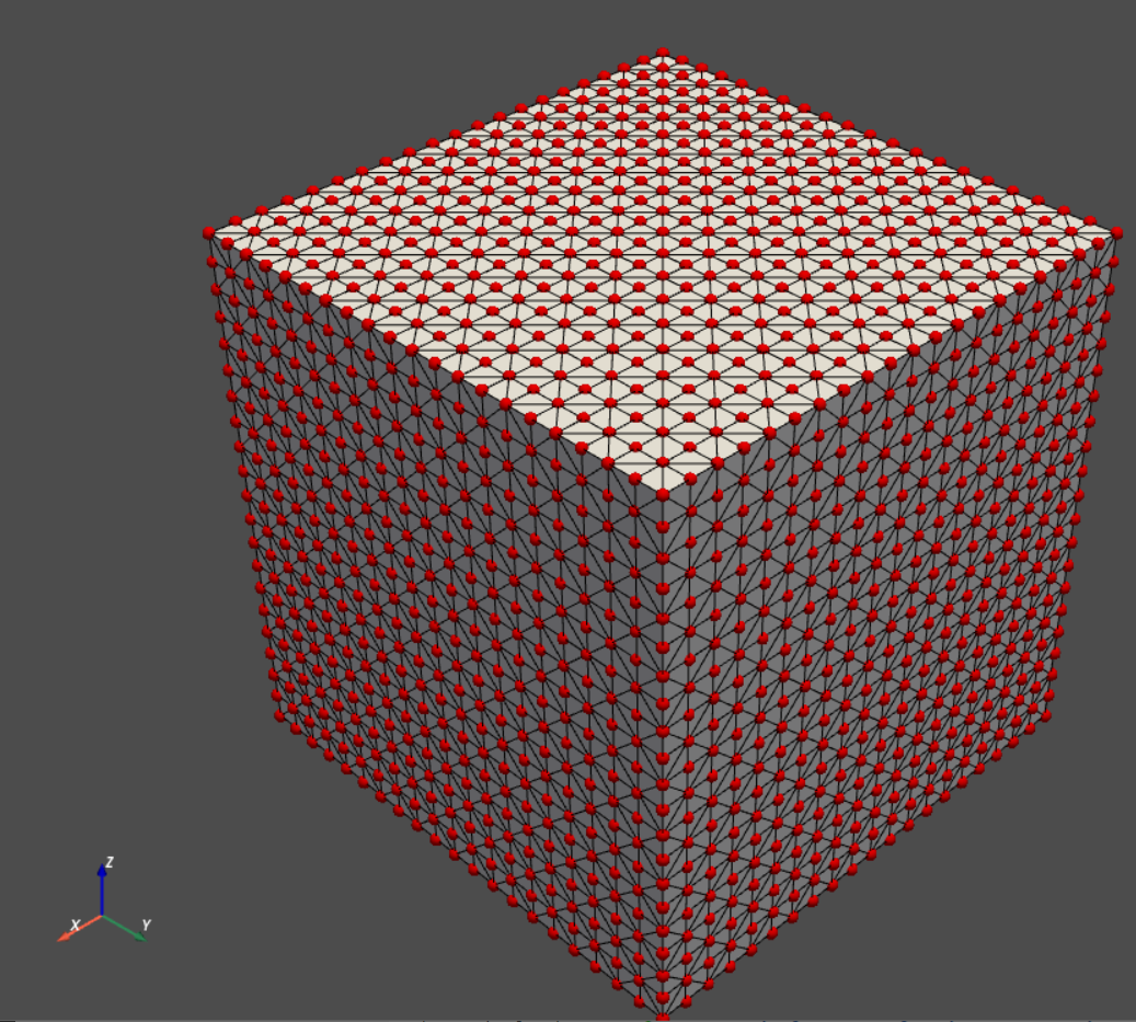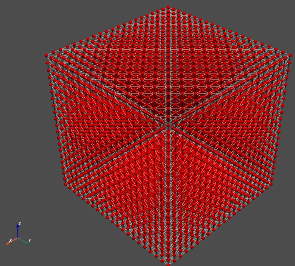There are other utility functions such as visualize_scalar_on_fem_points, visualize_scalar_on_fvm_points, etc.