Static Linear Elasticity
The governing equation for static linear elasticity is
\[\begin{aligned} \mathrm{div}\ \sigma(u) &= f(x) & x\in \Omega \\ \sigma(u) &= C\varepsilon(u) \\ u(x) &= u_0(x) & x\in \Gamma_u\\ \sigma(x) n(x) &= t(x) & x\in \Gamma_n \end{aligned}\]
Here $\varepsilon(u) = \frac{1}{2}(\nabla u + (\nabla u)^T)$ is the Cauchy tensor, $\Gamma_u \cup \Gamma_n = \Omega$, $\Gamma_u \cap \Gamma_n = \emptyset$. The weak formulation is: finding $u$ such that
\[\int_\Omega \delta \varepsilon(u) : C \varepsilon(u)\mathrm{d} x = \int_{\Gamma_n} t\cdot\delta u \mathrm{d}s - \int_\Omega f\cdot \delta u \mathrm{d}x\]
The codes for conducting linear elasticity problem can be here.
To verify our program, we first consider a parameter inverse problem where $E$ is a constant parameter that does not depend on $\mathbf{x}$. Additionally, we also let $\nu$ be an unknown parameter. We generate the displacement data using $E = 1.5$, $\nu = 0.3$. In the inverse problem, all displacement data are used to learn the parameters $E$ and $\nu$. The following table shows the learned parameters $E$ and $\nu$. We can see that our algorithm is quite efficient: after around 11 iterations, we reduce the absolute error to an order of $10^{-12}$ and $10^{-11}$ for $E$ and $\nu$, respectively.
| Parameter | Initial Guess | Learned | Exact | Absolute Error |
|---|---|---|---|---|
| $E$ | 1.0 | 1.5 | 1.5 | $6.04\times 10^{-12}$ |
| $\nu$ | 0.0 | 0.3 | 0.3 | $1.78\times 10^{-11}$ |
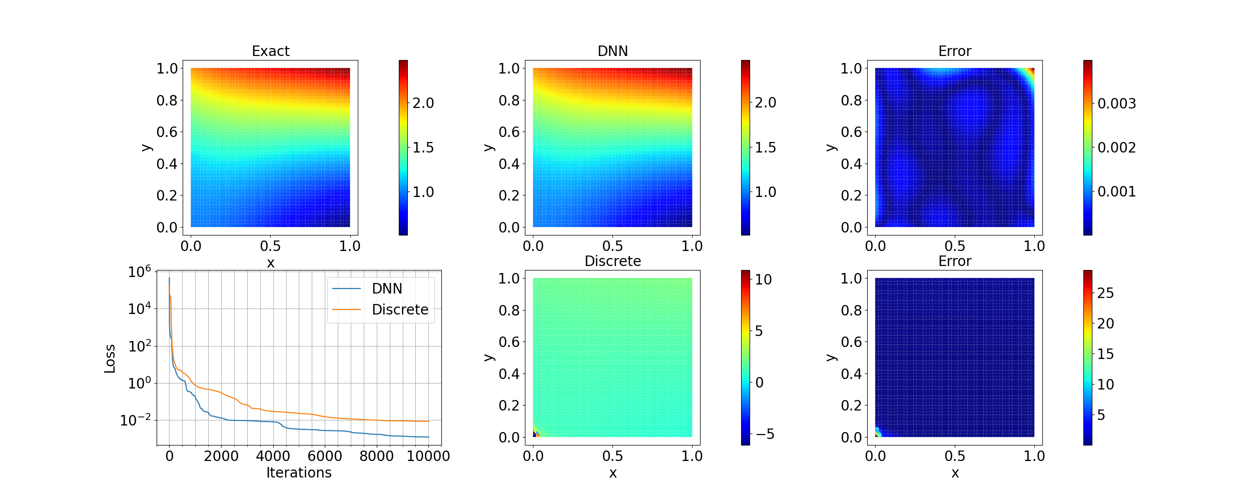
Next we consider a spatially-varying field $E(\mathbf{x})$ and fix $\nu=0.3$. We approaximate $E(\mathbf{x})$ using a deep neural network. The results are shown in the following figure. As a comparison, the result for representing $E(\mathbf{x})$ as a discrete vector of trainable variables is also shown. We can see that the DNN approach provides a much better result that the discretization approac