Perfectly Matched Layer

The code for this section can be found here.

Acosutic Wave Equation

In this example, we consider the finite element simulation for acoustic wave equations with perfectly matched layers (PML). The perfectly matched layer is a highly effecient absorbing boundary condition for numerical modeling of seismic wave equations. We consider the acoustic wave equation

\[u_{tt} = \nabla \cdot( c^2 \nabla u) + f \tag{1}\]

Here $c$ is the velocity. If a Dirichlet boundary condition is imposed, Eq. 1 will exhibit wave reflection on the boundary, which is an artifact of a finite computational domain.

To motive the perfectly matched layer, we consider Eq. 1 in the frequency domain

\[-\omega^2 \hat u = \nabla \cdot( c^2 \nabla \hat u) + \hat f \tag{2}\]

The homogeneous solution to Eq. 2 is

\[\hat u = A \exp[-i(k_1x + k_2y - \omega t)]\tag{3}\]

The idea is to let $\hat u$ "die out" near the boundary. Using complex analysis, Eq. 2 can be analytically extended to complex domain for both $x$ and $y$ (the complex numbers are denoted as $\tilde x$ and $\tilde y$)

\[\hat u = A \exp[-i(k_1\tilde x + k_2\tilde y - \omega t)]\tag{3}\]

Let us consider the $+x$ direction, instead of looking at the real axis, we consider the transformation

\[\tilde x = x - \frac{i}{\omega}\int_0^x \beta(s) ds, \tilde y = y\]

and thus

\[\hat u = A \exp[-i(k_1 (x - \frac{i}{\omega}\int_0^\beta \beta(s) ds) + k_2y - \omega t)] = A \exp[-i(k_1 x + k_2y - \omega t)]\exp\left(- \frac{1}{\omega}\int_0^x \beta(s) ds) \right)\]

Here $\exp\left(- \frac{1}{\omega}\int_0^x \beta(s) ds) \right)$ serves as the decaying factor.

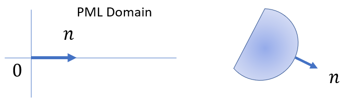
In the more general case, we replace the $+x$ direction with the outward normal direction (inside the domain, the outward normal can be defined as any unit vector).

\[\tilde n(n) = n - \frac{i}{\omega}\int_0^n \beta(s) ds, \tilde y = y\]

To derive the governing equation in terms of $n$ using the governing equation in terms of $\tilde n$, note that

\[\frac{\partial n}{\partial \tilde n} = \frac{i \omega}{i\omega + \beta(n)}\tag{4}\]

and

\[\nabla = n\partial_n + \nabla^\parallel\tag{5}\]

Here $\partial_n = n^T\nabla$ and $\nabla^\parallel = (I - nn^T)\nabla$. Plug Eq. 4 and Eq. 5 into (the arguments are $\tilde x$ and $\tilde y$)

\[-\omega^2 \hat u = \nabla \cdot( c^2 \nabla \hat u) + \hat f \tag{6}\]

we arrive at the equation

\[\begin{aligned}-\omega^2 \hat u &\\ = & n\partial_n \cdot(c^2 n\partial_n \hat u) (\partial n/\partial \tilde n)^2 \\ & + n\cdot (c^2n\partial_n \hat u)(\partial n/\partial \tilde n)\partial_n(\partial n/\partial \tilde n)\\ &+[n\partial_n \cdot(c^2 \nabla^\parallel \hat u) + \nabla^\parallel \cdot (c^2 n\partial_n \hat u)] (\partial n/\partial \tilde n) \\ &+ \nabla^\parallel \cdot(c^2 \nabla^\parallel\hat u) \end{aligned}\]

We can decompose $u$ into 4 parts:

\[\hat u = \hat u_1 + \hat u_2 + \hat u_3 + \hat u_4\]

and thus

\[\begin{aligned}-\omega^2 \hat u_1 &= n\partial_n \cdot(c^2n\partial_n \hat u)(\partial n/\partial \tilde n)^2\\ -\omega^2 \hat u_2 &= n\cdot (c^2n\partial_n \hat u)(\partial n/\partial \tilde n)\partial_n(\partial n/\partial \tilde n)\\ -\omega^2 \hat u_3 &=[n\partial_n \cdot(c^2 \nabla^\parallel \hat u) + \nabla^\parallel \cdot (c^2 n\partial_n \hat u)] (\partial n/\partial \tilde n)\\ -\omega^2 \hat u_4 &=\nabla^\parallel \cdot(c^2 \nabla^\parallel\hat u) \end{aligned}\]

This translates to the equations in the time domain

\[\begin{aligned}(\partial_t + \beta)^2 u_1 &= n\partial_n \cdot(c^2n\partial_n u)\\ (\partial_t + \beta)^3 u_2 &= -\beta' n\cdot (c^2n\partial_n u)\\ \partial_t(\partial_t + \beta) u_3 &=[n\partial_n \cdot(c^2 \nabla^\parallel u) + \nabla^\parallel \cdot (c^2 n\partial_n u)] \\ \partial_t^2 u_4 &=\nabla^\parallel \cdot(c^2 \nabla^\parallel u) \end{aligned}\tag{7}\]

We can introduce an intermediate variable

\[t = (\partial_t + \beta)u_2\tag{8}\]

and thus we have

\[(\partial_t + \beta)^2 t = -\beta' n\cdot (c^2n\partial_n u)\]

Eq. 7 is solved using FEM (see ExplicitNewmark) and equation is solved using a second-order Runge-Kutta method.

This numerical scheme is taken from

Zhao, Jian-Guo, and Rui-Qi Shi. "Perfectly matched layer-absorbing boundary condition for finite-element time-domain modeling of elastic wave equations." Applied Geophysics 10.3 (2013): 323-336.

Acosutic Wave Equation Examples

The following shows the results of the numerical scheme introduced in the last section.

Domain	Without PML	With PML
Square
Disk

Elastic Wave Equation

We now consider the elastic wave equation.

\[\ddot\mathbf{u} = \nabla \cdot (C : \nabla \mathbf{u})\tag{9}\]

Here $C$ is the elastic tensor and : is a contraction operator, which is defined as follows

\[C:\nabla \mathbf{u} = \bm{\sigma} := \begin{bmatrix}\sigma_{xx} & \sigma_{xy} \\ \sigma_{yx} & \sigma_{yy}\end{bmatrix}\]

Here the stress tensor is computed using

\[\begin{bmatrix}\sigma_{xx}\\\sigma_{yy}\\\sigma_{xy}\end{bmatrix} = \begin{bmatrix}\lambda+2\mu & \lambda &0.0\\\lambda & \lambda+2\mu &0.0\\0 & 0 & \mu\end{bmatrix}\begin{bmatrix}\varepsilon_{xx} \\ \varepsilon_{yy} \\ 2\varepsilon_{xy}\end{bmatrix}\]

where the strain tensor is defined as

\[\bm{\varepsilon} := \begin{bmatrix}\varepsilon_{xx} & \varepsilon_{xy} \\\varepsilon_{xy} & \varepsilon_{yy} \end{bmatrix} = \begin{bmatrix}u_x & \frac{u_y+v_x}{2} \\\frac{u_y+v_x}{2} & v_y \end{bmatrix}\]

The weak form of the right hand side of Eq. 9 (up to the sign), we have

\[\begin{aligned}& \langle C: \nabla \mathbf{u}, \nabla \mathbf{u}'\rangle \\ =& \begin{bmatrix} u_x' & u_y' & v_x' & v_y'\end{bmatrix}\begin{bmatrix}1 &0 &0 \\ 0 &0 &1\\0 & 0 & 1\\0 & 1 &0\end{bmatrix} \begin{bmatrix} a&b&0\\b&a&0\\0&0&c \end{bmatrix} \begin{bmatrix}1 & 0 & 0 &0 \\ 0 &0 &0 &1 \\0 & 1 & 1 &0\end{bmatrix} \begin{bmatrix} u_x \\ u_y \\ v_x \\ v_y\end{bmatrix}\\ =& \begin{bmatrix} u_x' & u_y' & v_x' & v_y'\end{bmatrix} \begin{bmatrix}a & 0 & 0 & b\\ 0 & c & c & 0\\ 0 & c & c & 0\\ b & 0 & 0 & a\end{bmatrix} \begin{bmatrix} u_x \\ u_y \\ v_x \\ v_y\end{bmatrix}\end{aligned}\tag{10}\]

Here

\[a = \lambda + 2\mu, \quad b = \lambda, \quad c = \mu\]

\[\langle C: \nabla \mathbf{u}, \nabla u'\rangle = \begin{bmatrix}u_x'&u_y'&u_z'&v_x'&v_y'&v_z'&w_x'&w_y'&w_z'\end{bmatrix}\begin{bmatrix} a & 0 & 0 & 0 & b & 0 & 0 & 0 & b\\0 & c & 0 & c & 0 & 0 & 0 & 0 & 0\\0 & 0 & c & 0 & 0 & 0 & c & 0 & 0\\0 & c & 0 & c & 0 & 0 & 0 & 0 & 0\\ b & 0 & 0 & 0 & a & 0 & 0 & 0 & b\\0 & 0 & 0 & 0 & 0 & c & 0 & c & 0\\0 & 0 & c & 0 & 0 & 0 & c & 0 & 0\\0 & 0 & 0 & 0 & 0 & c & 0 & c & 0\\ b & 0 & 0 & 0 & b & 0 & 0 & 0 & a\end{bmatrix}\begin{bmatrix}u_x\\u_y\\u_z\\v_x\\v_y\\v_z\\w_x\\w_y\\w_z\end{bmatrix}\]

We can use Eq. 7 for simulation, except that we replace $c^2$ with the elastic tensor operation $C$.

Variable	Without PML	With PML
$u$
$v$