Unstructured Meshes in AdFem

AdFem.jl also provides unstructured mesh support by leveraging MFEM as the finite element backend.

The APIs are designed such that they are consistent with structured meshes. For most of the functions, we only need to replace geometry parameters m, n, h with mesh, which is a Mesh instance. The triangular elements are the default in the AdFem unstructured mesh module. Mesh can be constructed using a $N\times 2$ node vector and a $E\times 3$ element vector (1-based); for example:

nodes = [0.0 0.0;1.0 0.0;0.0 1.0;1.0 1.0]
elems = [1 2 3;2 3 4]
mesh = Mesh(nodes, elems)

Particularly, we provide a convenient constructor for constructing meshes on a rectangle:

mesh = Mesh(m, n, h)
visualize_mesh(mesh)

Because we do not use the static condensation technique for tackling boundary conditions, there is no need to specify boundary conditions at this point. Plus, the lack of boundary conditions make it easier to develope re-usable custom operators for the finite element method.

The following script shows how to use an unstructured mesh to solve the Poisson equation here

using PyPlot 
using AdFem

m = 50; n = 50; h = 1/n 
mesh = Mesh(m, n, h)
kappa = constant(ones(get_ngauss(mesh)))
A = compute_fem_laplace_matrix1(kappa, mesh)
F = constant(eval_f_on_gauss_pts((x,y)->2π^2*sin(π*x)*sin(π*y), mesh))

bd = Int64[]
for j = 1:m+1
    push!(bd, j)
    push!(bd, n*(m+1)+j)
end
for i = 2:n
    push!(bd, (i-1)*(m+1)+1)
    push!(bd, (i-1)*(m+1)+m+1)
end

A, _ = fem_impose_Dirichlet_boundary_condition1(A, bd, mesh)
rhs = compute_fem_source_term1(F, mesh)
rhs = scatter_update(rhs, bd, zeros(length(bd)))
sol = A\rhs

sess = Session(); init(sess)
S = run(sess, sol)

figure(figsize=(10,4))
subplot(121)
visualize_scalar_on_fem_points(S, mesh)
title("Computed")
subplot(122)
visualize_scalar_on_fem_points(eval_f_on_fem_pts((x,y)->sin(π*x)*sin(π*y), mesh), mesh)
title("Reference")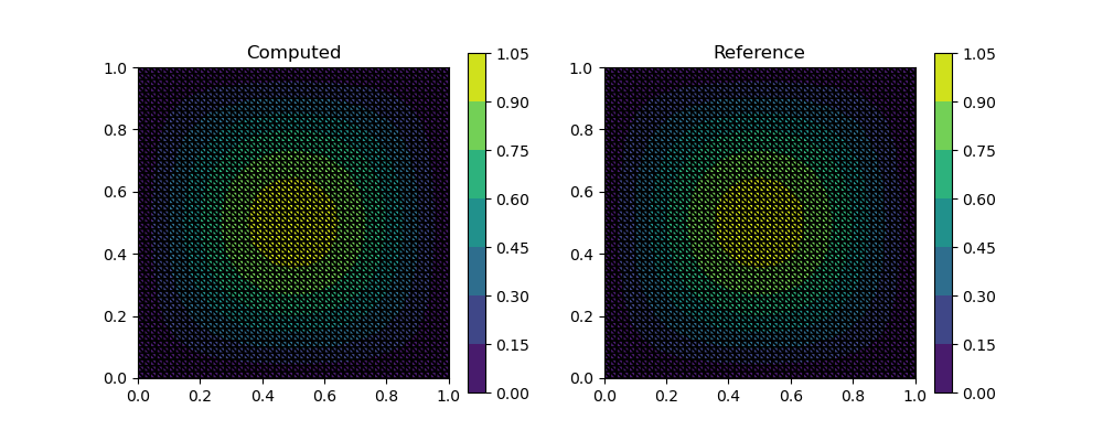

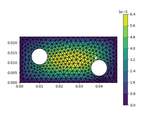
As a more interesting example, we consider the domain with two holes. Here we let the right hand side be 1. We impose Dirichlet boundary conditions on the bounding box and Neumann boundary conditions around the disc boundaries.

using PyPlot 
using AdFem

mesh = Mesh("twoholes.msh")

kappa = constant(ones(get_ngauss(mesh)))
A = compute_fem_laplace_matrix1(kappa, mesh)
F = constant(eval_f_on_gauss_pts((x,y)->1.0, mesh))

bd = Int64[]
for i = 1:size(mesh.nodes, 1)
    x = mesh.nodes[i,1]
    y = mesh.nodes[i,2]
    if abs(x-0.049)<1e-5 || abs(x)<1e-5 || abs(y)<1e-5 || abs(y-0.023)<1e-5
        push!(bd, i)
    end
end

A, _ = fem_impose_Dirichlet_boundary_condition1(A, bd, mesh)
rhs = compute_fem_source_term1(F, mesh)
rhs = scatter_update(rhs, bd, zeros(length(bd)))
sol = A\rhs

sess = Session(); init(sess)
S = run(sess, sol)

visualize_scalar_on_fem_points(S, mesh)
savefig("uPoisson.png")