Adding Custom Operators for Unstructured Meshes

Workflow

This tutorial describes how to develop custom operators for unstructured meshes.

AdFem uses MFEM as the backend for assembling finite element matrices. However, users, as well as custom operator developers, do not need to know how to use MFEM. AdFem has provided an easier interface to essential data structures for assembling finite element matrices. The data structure can be assessed in C++ (see Mesh) and the header files are located in deps/MFEM/Common.h. As the structured mesh utilties, we do not expose the APIs for Julia users, and therefore if some operators are lacking, users must modify the source codes of AdFem.

The basic workflow is to go into deps/MFEM directory. Then

Make a new directory to add all source codes related to your custom operator.
Generate templated files using customop.
In your source code, do remember to include ../Common.h, which exposes mmesh for all necessary data structures.
Add your source code file names to deps/MFEM/CMakeLists.txt.
Recompile AdFem or run ninja in deps/MFEM/build.
Test your code. Note you need to replace the library path in load_op_and_grad by AdFem.libmfem in order to share the same mmesh throughout the session.

Assembling Matrices and Vectors

The main approach for assembling matrices and vectors in finite element methods is to loop over each element (triangles in our case), and computes contributions to the corresponding local degrees of freedom (DOF). For example, for P1 (linear) element, the local DOFs are three vertices; for P2 (quadratic) element, the local DOFs are both vertices and edges.

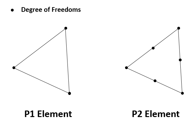
Each finite element (triangle) is represented by NNFEM_Element in the C++ shared library of AdFem. The local DOFs are mapped to global DOFs via dof array, which is a 6-dimensional array. For P1 element, the last three components are redundant. For P2 elements, the global indices are arranged in a way such that all edge indices are after the nodal indices. The mapping between edge indices and vertices can be found in edges in the structure Mesh.

When we loop over each element, each DOF is associated with a basis function $\phi_i(x, y)$, such that $\phi_i(x_j, y_j) = \delta_{ij}$, where $(x_j, y_j)$ is the nodes shown in the above plots. For convenience, an element (NNFEM_Element) provides the values of

\[\phi_i(\tilde x_k, \tilde y_k), \partial_x \phi_i(\tilde x_k, \tilde y_k), \partial_y \phi_i(\tilde x_k, \tilde y_k), \tilde\phi_i(\tilde x_k, \tilde y_k) \tag{1}\]

Here $(\tilde x_k, \tilde y_k)$ is the $k$-th Guass points for the current element, and $\tilde \phi_i$ is the basis function for P1 element. The data are stored in h, hx, hy, hs respectively. Additionally, the element also contains a weight vector w that stores the quadrature weights (adjusted by triangle areas). Note Equation 1 are all physical shape functions. Therefore, we can conveniently compute many quantities. For example, if we want to compute $\int_A \nabla u \cdot \nabla v dx dy$ on the element $A$ ($u$ is the trial function, and $v$ is the test function), $\int_A \nabla \phi_i \cdot \nabla \phi_j dxdy$ can be expressed as

double s = 0.0;
for (int r = 0; r < elem->ngauss; r++){
    s += ( elem->hx(i, r) * elem->hx(j, r) + elem->hy(i, r) * elem->hy(j, r)) * elem->w(r);
}

The corresponding indices in the global sparse matrix is

int I = elem->dof[i];
int J = elem->dof[j];`

For the quadratic element, it has 6 DOFs for each element

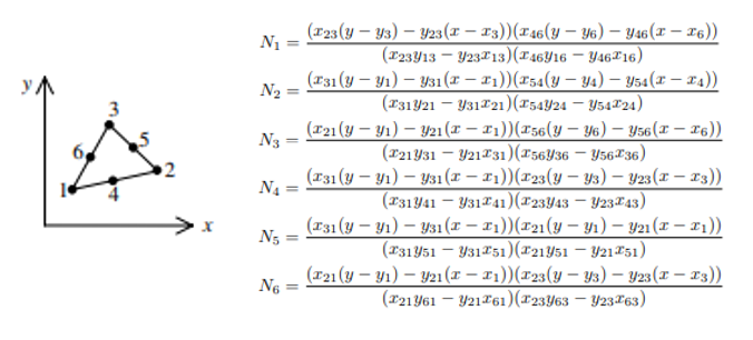
Here $x_{ij} = x_i - x_j$, $y_{ij} = y_i - y_j$. We can use this information to assemble linear or bilinear forms. For example, in the course of implementing compute_fem_traction_term1, we can first extract quadrature rules using

IntegrationRules rule_;
IntegrationRule rule = rule_.Get(Element::Type::SEGMENT, order);
const IntegrationPoint &ip = rule.IntPoint(i)

Then we have access to ip.weight and ip.x.

Verifying Implementation against FEniCS

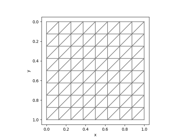
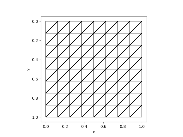
To test unstructured meshes, we can compare the results with fenics. We can use the same mesh:

mesh = Mesh(8, 8, 1/8)

The corresponding Python code is

mesh = UnitSquareMesh(8, 8, "left")

FEniCS	AdFem

As an example, in deps/MFEM/ComputeInteractionTerm, we developed a custom operator to compute $\int_\Omega p \begin{bmatrix}\frac{\partial u}{\partial x} \\\frac{\partial u}{\partial y}\end{bmatrix} dx$ We can compute the values using FEniCS

from __future__ import print_function
from fenics import *
import matplotlib.pyplot as plt
import numpy as np 

# Create mesh and define function space
mesh = UnitSquareMesh(8, 8, "left")
P = FunctionSpace(mesh, 'DG', 0)
U = FunctionSpace(mesh, "CG", 1)

# Define variational problem
u = TrialFunction(U)
p = TestFunction(P)
a = dot(p, u.dx(0))*dx
b = dot(p, u.dx(1))*dx


A = assemble(a).array().T
x = np.random.random((A.shape[1],))
f = np.dot(A, x)
A1 = assemble(b).array().T
f1 = np.dot(A1, x)
DofToVert = vertex_to_dof_map(u.function_space())

np.savetxt("fenics/f.txt", np.concatenate([f[DofToVert], f1[DofToVert]]))
np.savetxt("fenics/x.txt", x)

The corresponding Julia code is

using ADCME
using LinearAlgebra
using AdFem
using DelimitedFiles

p = readdlm("fenics/x.txt")[:]
f = readdlm("fenics/f.txt")[:]

mesh = Mesh(8, 8, 1. /8)
f0 = compute_interaction_term(p, mesh)
sess = Session(); init(sess)
f1 = run(sess, f0)

@show norm(f - f1)

We get the result:

norm(f - f1) = 3.0847790632031627e-16

Install FEniCS

It is recommend to install FEniCS by creating a new conda environment. For example, on a Linux server, you can do

conda create -n fenicsproject -c conda-forge fenics
source activate fenicsproject

Please refer to built-in AdFem custom operators to see how FEniCS is used for validation.