Mixed Finite Element Methods for Poisson's Equation

In this section, we consider solving the Poisson's equation using mixed finite element methods

\[-\nabla \cdot (\nabla u(x)) = f \text{ in } \Omega\tag{1}\]

with boundary conditions

\[u = g_D \text{ on } \partial \Omega\]

We reformulate the Eq. 1 as

\[\begin{aligned}\sigma + \nabla u &= 0 \\ \nabla \cdot \sigma & = f \end{aligned}\]

The mixed variational formulation is to find $(\sigma, u)\in H(\text{div}, \Omega) \times L^2(\Omega)$, such that

\[\begin{aligned}(\sigma, \tau) - (\nabla \cdot \tau, u) &= -(\tau\cdot \mathbf{n}, g_D)_{\partial \Omega}\\ (\nabla \cdot \sigma, v) &= (f, v)\end{aligned}\]

We use the following stable pair of elements: BDM${}_1$-P${}_0$, where the stress space is approximated using a BDM element while the displacement space is approximated using a piecewise constant element.

The code is as follows:

# Solves the Poisson equation using the Mixed finite element method 
using Revise
using AdFem
using DelimitedFiles
using SparseArrays
using PyPlot


n = 50
mmesh = Mesh(n, n, 1/n, degree = BDM1)

testCase = [
    ((x, y)->begin
        x * (1-x) * y * (1-y)
    end, 
    (x, y)->begin
        -2x*(1-x) -2y*(1-y)
    end),  # test case 1
    ((x, y)->begin
        x^2 * (1-x) * y * (1-y)^2
    end, 
    (x, y)->begin
        2*x^2*y*(1 - x) + 2*x^2*(1 - x)*(2*y - 2) - 4*x*y*(1 - y)^2 + 2*y*(1 - x)*(1 - y)^2
    end) ,# test case 2
    (
        (x, y)->x*y, 
        (x, y)->0.0
    ), # test case 3
    (
        (x, y)->x^2 * y^2 + 1/(1+x^2), 
        (x, y)->2*x^2 + 8*x^2/(x^2 + 1)^3 + 2*y^2 - 2/(x^2 + 1)^2
    ), # test case 4
]

for k = 1:4
    @info "TestCase $k..."
    ufunc, ffunc = testCase[k]

    A = compute_fem_bdm_mass_matrix1(mmesh)
    B = compute_fem_bdm_div_matrix1(mmesh)
    C = [A -B'
        -B spzeros(mmesh.nelem, mmesh.nelem)]

    gD = bcedge(mmesh)
    t1 = eval_f_on_boundary_edge(ufunc, gD, mmesh)
    g = compute_fem_traction_term1(t1, gD, mmesh) 
    t2 = eval_f_on_gauss_pts(ffunc, mmesh)
    f = compute_fvm_source_term(t2, mmesh)
    rhs = [-g; f]

    sol = C\rhs
    u = sol[mmesh.ndof+1:end]
    close("all")
    figure(figsize=(15, 5))
    subplot(131)
    title("Reference")
    xy = fvm_nodes(mmesh)
    x, y = xy[:,1], xy[:,2]
    uf = ufunc.(x, y)
    visualize_scalar_on_fvm_points(uf, mmesh)
    subplot(132)
    title("Numerical")
    visualize_scalar_on_fvm_points(u, mmesh)
    subplot(133)
    title("Absolute Error")
    visualize_scalar_on_fvm_points( abs.(u - uf) , mmesh)
    savefig("bdm$k.png")
end

Here we have 4 test cases, and we show the results for each test case:

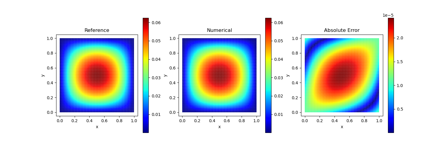
Test Case 1

Analytical solution:

\[u(x, y) = x(1-x)y(1-y)\]

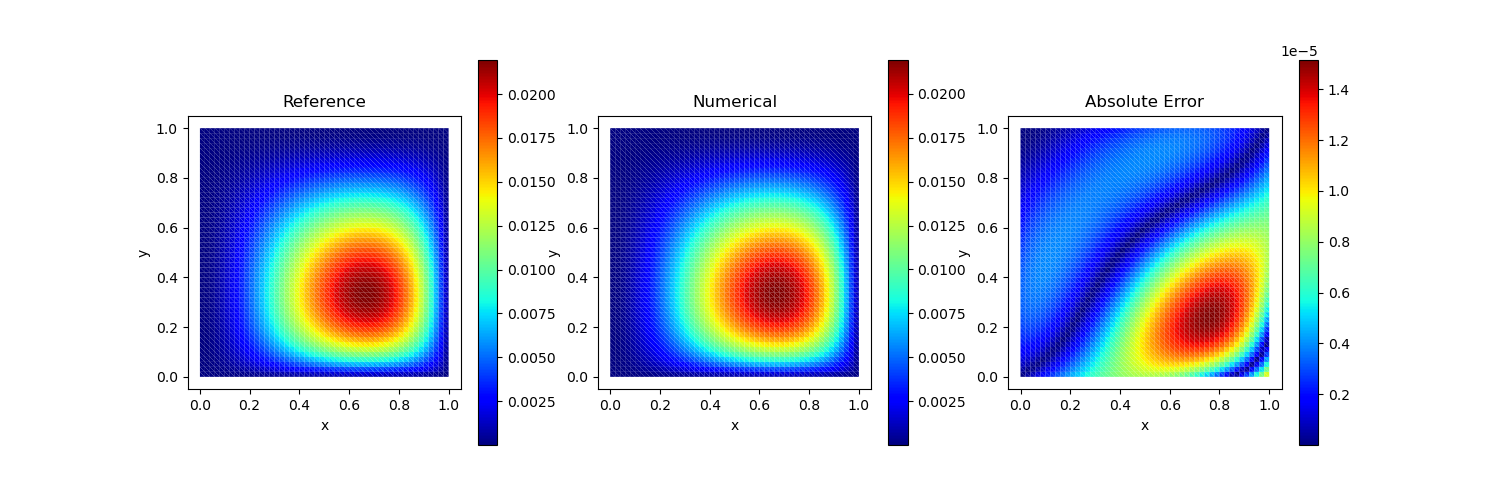
Test Case 2

Analytical solution:

\[u(x, y) = x^2 (1-x) y (1-y)^2\]

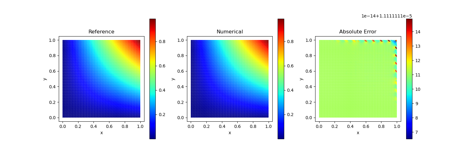
Test Case 3

Analytical solution:

\[u(x, y) = xy\]

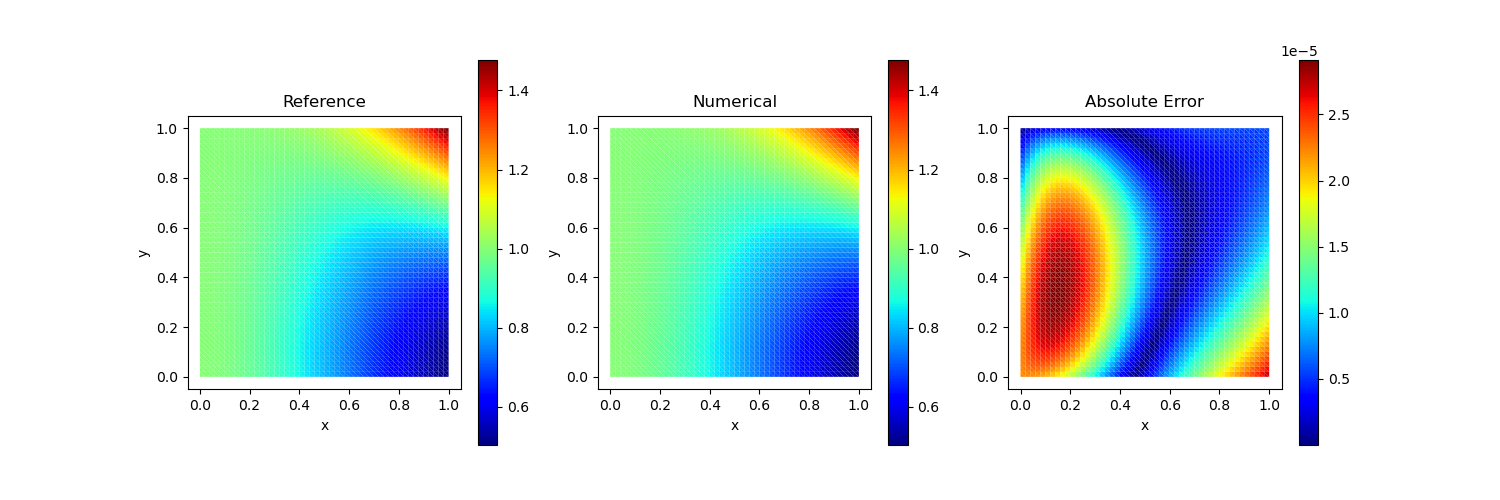
Test Case 4

\[u(x,y) = x^2 y^2 + \frac{1}{1+x^2}\]

Traction Boundary Condition

We consider the case where the boundary conditions are given by

\[\sigma \cdot \mathbf{n} = g_N, x\in \Gamma_N, \quad u = g_D, x\in \Gamma_D\]

The weak form is

\[\begin{aligned}(\sigma, \tau) - (\nabla \cdot \tau, u) &= -(\tau\cdot \mathbf{n}, g_D)_{\Gamma_D}\\ (\nabla \cdot \sigma, v) &= (f, v)\end{aligned}\]

In this case, the traction boundary condition does not appear in the weak form, but determines the coefficients for the representation of $\sigma$ for the DOFs on the boundary $\Gamma_N$. Consider an edge $E_l = \{e_s, e_t\}, s<t$, then we have

\[\sigma = a\phi_{l,1} + b \phi_{l, 2}\]

which leads to

\[|E_l|g_N = a \lambda_s + b \lambda_t\]

To calculate $a, b$, we solve the following linear system

\[\begin{bmatrix}(\lambda_s, \lambda_s) & (\lambda_s, \lambda_t) \\ (\lambda_s, \lambda_t) & (\lambda_t, \lambda_t)\end{bmatrix}\begin{bmatrix}a\\b\end{bmatrix} = |E_l|\begin{bmatrix}(g_N, \lambda_s)\\ (g_N, \lambda_t)\end{bmatrix}\]

The boundary condition can be computed using impose_bdm_traction_boundary_condition1.

# Solves the Poisson equation using the Mixed finite element method 
using Revise
using AdFem
using DelimitedFiles
using SparseArrays
using PyPlot


n = 50
mmesh = Mesh(n, n, 1/n, degree = BDM1)

function ufunc(x, y)
    x * (1-x) * y * (1-y)
end

function ffunc(x, y)
    -2x*(1-x) -2y*(1-y)
end

function gfunc(x, y)
    (1-2x)*y*(1-y)
end

A = compute_fem_bdm_mass_matrix1(mmesh)
B = compute_fem_bdm_div_matrix1(mmesh)
C = [A -B'
    -B spzeros(mmesh.nelem, mmesh.nelem)]

gD = (x1, y1, x2, y2)->!( (x1<1e-3 && y1>1e-3 && y1<1-1e-3) ||  (x2<1e-3 && y2>1e-3 && y2<1-1e-3))
gN = (x1, y1, x2, y2)->x1<1e-5 && x2<1e-5

D_bdedge = bcedge(gD, mmesh)
N_bdedge = bcedge(gN, mmesh)

t1 = eval_f_on_boundary_edge(ufunc, D_bdedge, mmesh)
g = compute_fem_traction_term1(t1, D_bdedge, mmesh) 
t2 = eval_f_on_gauss_pts(ffunc, mmesh)
f = compute_fvm_source_term(t2, mmesh)

gN = eval_f_on_boundary_edge(gfunc, N_bdedge, mmesh)
dof, val = impose_bdm_traction_boundary_condition1(gN, N_bdedge, mmesh)
rhs = [-g; f]
C, rhs = impose_Dirichlet_boundary_conditions(C, rhs, dof, val)

sol = C\rhs
u = sol[mmesh.ndof+1:end]
close("all")
figure(figsize=(15, 5))
subplot(131)
title("Reference")
xy = fvm_nodes(mmesh)
x, y = xy[:,1], xy[:,2]
uf = ufunc.(x, y)
visualize_scalar_on_fvm_points(uf, mmesh)
subplot(132)
title("Numerical")
visualize_scalar_on_fvm_points(u, mmesh)
subplot(133)
title("Absolute Error")
visualize_scalar_on_fvm_points( abs.(u - uf) , mmesh)
savefig("mixed_poisson_neumann.png")

The result is shown below