Generalized α Scheme
Generalized $\alpha$ Scheme
The generalized $\alpha$ scheme is used to solve the second order linear differential equation of the form
\[m\ddot{ \mathbf{u}} + \gamma\dot{\mathbf{u}} + k\mathbf{u} = \mathbf{f}\]
whose discretization form is
\[M\mathbf{a} + C\mathbf v + K \mathbf d = \mathbf F\]
Here $M$, $C$ and $K$ are the generalized mass, damping, and stiffness matrices, $\mathbf a$, $\mathbf v$, and $\mathbf d$ are the generalized acceleration, velocity, and displacement, and $\mathbf F$ is the generalized force vector.
There are two types of boundary conditions
- Dirichlet (essential) boundary condition. In this case, the displacement $\mathbf{u}$ is specified at a point $\mathbf{x}_0$
\[\mathbf{u}(\mathbf{x}_0, t) = \mathbf{h}(t)\]
This boundary condition usually requires updating matrices $M$, $C$ and $K$ at each time step.
- Essential boundry condition. In this case the external force is specified
\[{\sigma}(\mathbf{x})\mathbf{n}(\mathbf{x}) = \mathbf{t}(\mathbf{x})\]
This term goes directly into $\mathbf{F}$.
The generalized $\alpha$ scheme solves for a discrete time step
\[\begin{aligned} \mathbf d_{n+1} &= \mathbf d_n + h\mathbf v_n + h^2 \left(\left(\frac{1}{2}-\beta_2 \right)\mathbf a_n + \beta_2 \mathbf a_{n+1} \right)\\ \mathbf v_{n+1} &= \mathbf v_n + h((1-\gamma_2)\mathbf a_n + \gamma_2 \mathbf a_{n+1})\\ \mathbf F(t_{n+1-\alpha_{f_2}}) &= M \mathbf a _{n+1-\alpha_{m_2}} + C \mathbf v_{n+1-\alpha_{f_2}} + K \mathbf{d}_{n+1-\alpha_{f_2}} \end{aligned}\]
Here $h$ is the time step and
\[\begin{aligned} \mathbf d_{n+1-\alpha_{f_2}} &= (1-\alpha_{f_2})\mathbf d_{n+1} + \alpha_{f_2} \mathbf d_n\\ \mathbf v_{n+1-\alpha_{f_2}} &= (1-\alpha_{f_2}) \mathbf v_{n+1} + \alpha_{f_2} \mathbf v_n \\ \mathbf a_{n+1-\alpha_{m_2} } &= (1-\alpha_{m_2}) \mathbf a_{n+1} + \alpha_{m_2} \mathbf a_n\\ t_{n+1-\alpha_{f_2}} & = (1-\alpha_{f_2}) t_{n+1 + \alpha_{f_2}} + \alpha_{f_2}t_n \end{aligned}\]
The parameters $\alpha_{f_2}$, $\alpha_{m_2}$, $\gamma_2$, and $\beta_2$ are used to control the amplification of high frequency numerical modes. High frequency modes normally describe motions with no physical sense (also contains very large phase error). Therefore, it is desirable to damp those high frequency modes. By properly choosing the parameters, we can recover HHT, Newmark, or WBZ methods.
We can design new algorithms by taking $\rho_\infty\in [0,1]$ as a design variable to control the numerical dissipation above the normal frequency $\frac{h}{T}$, where $T$ is the period associated with the highest frequency of interest. The following relationships are used to obtain a good algorithm that are accurate and preserve low-frequency modes
\[\begin{aligned} \gamma_2 &= \frac{1}{2} - \alpha_{m_2} + \alpha_{f_2}\\ \beta_2 &= \frac{1}{4} (1-\alpha_{m_2}+\alpha_{f_2})^2 \\ \alpha_{m_2} &= \frac{2\rho_\infty-1}{\rho_\infty+1}\\ \alpha_{f_2} &= \frac{\rho_\infty}{\rho_\infty+1} \end{aligned}\]
The following figure provides a plot of spectral radii versus $\frac hT$[radii]

In ADCME, we provide an API to the generalized $\alpha$ scheme, αscheme, and αscheme_time, which computes $t_{n+1-\alpha_{f_2}}$.
Rayleigh Damping
Rayleigh damping is widely used to model internal structural damping. It is viscous damping that is proportional to a linear combination of mass and stiffness
\[C = \alpha M + \beta K\]
The relation between the damping value $\xi$ and the naturual frequency $\omega$ is given by
\[\xi =\frac12\left( \frac{\alpha}{\omega} + \beta\omega \right)\]
In practice, we can measure two real frequencies $\xi_1$ and $\xi_2$, corresponding to $\omega_1$ and $\omega_2$ and find the coefficients via
\[\begin{bmatrix} \frac{1}{2\omega_1} & \frac{\omega_1}{2}\\ \frac{1}{2\omega_2} & \frac{\omega_2}{2} \end{bmatrix}\begin{bmatrix}\alpha\\\beta\end{bmatrix} = \begin{bmatrix}\xi_1\\\xi_2\end{bmatrix}\]
This approach will produce a curve that matches the two natural frequency points. In the case where the structure has one or two very dominant frequencies, Raleigh damping can closely approximate the behavior of a prescribed modal damping.
Example: Elasticity
In this example, we consider a plane stress elasticity deformation of a plate. The governing equation is given by
\[\begin{aligned} \sigma_{ij,j} + f_i = \ddot u_i \\ \sigma_{ij} = \mathsf{C} \epsilon_{ij} \end{aligned}\]
The elasticity tensor $\mathsf{C}$ is calculated using a Young's modulus $E=1$ and a Poisson's ratio $\nu=0.35$. We consider a computational domain $[0,2]\times[0,1]$ and time horizon $t\in (0,1)$, the exact solution is given by
\[u_1(x,y,t) = e^{-t}x(2-x)y(1-y)\qquad u_2(x,y,t) = e^{-t}x^2(2-x)^2y^2(1-y)^2\]
The other terms can be computed analytically based on the exact solutions.
using ADCME
using AdFem
using PyPlot
n = 20
m = 2n
NT = 200
ρ = 1.0
Δt = 1/NT
h = 1/n
x = zeros((m+1)*(n+1))
y = zeros((m+1)*(n+1))
for i = 1:m+1
for j = 1:n+1
idx = (j-1)*(m+1)+i
x[idx] = (i-1)*h
y[idx] = (j-1)*h
end
end
bd = bcnode("all", m, n, h)
u1 = (x,y,t)->exp(-t)*x*(2-x)*y*(1-y)
u2 = (x,y,t)->exp(-t)*x^2*(2-x)^2*y^2*(1-y)^2
ts = Δt * ones(NT)
dt = αscheme_time(ts, ρ = ρ )
F = zeros(NT, 2(m+1)*(n+1))
for i = 1:NT
t = dt[i]
f1 = (x,y)->(-4.93827160493827*x^2*y^2*(x - 2)*(y - 1) - 4.93827160493827*x^2*y*(x - 2)*(y - 1)^2 - 4.93827160493827*x*y^2*(x - 2)^2*(y - 1) - 4.93827160493827*x*y*(x - 2)^2*(y - 1)^2 + x*y*(x - 2)*(y - 1) - 0.740740740740741*x*(x - 2) - 3.20987654320988*y*(y - 1))*exp(-t)
f2 = (x,y)->(x^2*y^2*(x - 2)^2*(y - 1)^2 - 3.20987654320988*x^2*y^2*(x - 2)^2 - 0.740740740740741*x^2*y^2*(y - 1)^2 - 12.8395061728395*x^2*y*(x - 2)^2*(y - 1) - 3.20987654320988*x^2*(x - 2)^2*(y - 1)^2 - 2.96296296296296*x*y^2*(x - 2)*(y - 1)^2 - 1.23456790123457*x*y - 1.23456790123457*x*(y - 1) - 0.740740740740741*y^2*(x - 2)^2*(y - 1)^2 - 1.23456790123457*y*(x - 2) - 1.23456790123457*(x - 2)*(y - 1))*exp(-t)
fval1 = eval_f_on_gauss_pts(f1, m, n, h)
fval2 = eval_f_on_gauss_pts(f2, m, n, h)
F[i,:] = compute_fem_source_term(fval1, fval2, m, n, h)
end
E = 1.0
ν = 0.35
H = E/(1+ν)/(1-2ν)*[
1-ν ν 0
ν 1-ν 0
0 0 (1-2ν)/2
]
M = constant(compute_fem_mass_matrix(m, n, h))
K = constant(compute_fem_stiffness_matrix(H, m, n, h))
a0 = [(@. u1(x, y, 0.0)); (@. u2(x, y, 0.0))]
u0 = -[(@. u1(x, y, 0.0)); (@. u2(x, y, 0.0))]
d0 = [(@. u1(x, y, 0.0)); (@. u2(x, y, 0.0))]
function solver(A, rhs)
A, _ = fem_impose_Dirichlet_boundary_condition_experimental(A, bd, m, n, h)
rhs = scatter_update(rhs, [bd; bd .+ (m+1)*(n+1)], zeros(2*length(bd)))
return A\rhs
end
d, u, a = αscheme(M, spzero(2(m+1)*(n+1)), K, F, d0, u0, a0, ts; solve=solver, ρ = ρ )
sess = Session()
d_, u_, a_ = run(sess, [d, u, a])
function plot_traj(idx)
figure(figsize=(12,3))
subplot(131)
plot((0:NT)*Δt, u1.(x[idx], y[idx],(0:NT)*Δt), "b-", label="x-Acceleration")
plot((0:NT)*Δt, a_[:,idx], "y--", markersize=2)
plot((0:NT)*Δt, u2.(x[idx], y[idx],(0:NT)*Δt), "r-", label="y-Acceleration")
plot((0:NT)*Δt, a_[:,idx+(m+1)*(n+1)], "c--", markersize=2)
legend()
xlabel("Time")
ylabel("Value")
subplot(133)
plot((0:NT)*Δt, u1.(x[idx], y[idx],(0:NT)*Δt), "b-", label="x-Displacement")
plot((0:NT)*Δt, d_[:,idx], "y--", markersize=2)
plot((0:NT)*Δt, u2.(x[idx], y[idx],(0:NT)*Δt), "r-", label="y-Displacement")
plot((0:NT)*Δt, d_[:,idx+(m+1)*(n+1)], "c--", markersize=2)
legend()
xlabel("Time")
ylabel("Value")
subplot(132)
plot((0:NT)*Δt, -u1.(x[idx], y[idx],(0:NT)*Δt), "b-", label="x-Velocity")
plot((0:NT)*Δt, u_[:,idx], "y--", markersize=2)
plot((0:NT)*Δt, -u2.(x[idx], y[idx],(0:NT)*Δt), "r-", label="y-Velocity")
plot((0:NT)*Δt, u_[:,idx+(m+1)*(n+1)], "c--", markersize=2)
legend()
xlabel("Time")
ylabel("Value")
tight_layout()
end
idx2 = (n÷3)*(m+1) + m÷3
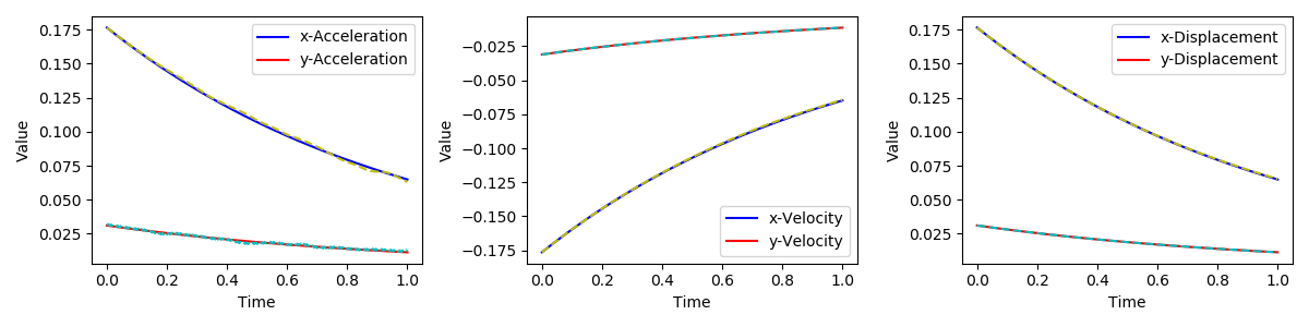
plot_traj(idx2)Using the above code, we plot the trajectories of $\mathbf{a}$, $\mathbf{v}$, and $\mathbf{d}$ at $(0.64,0.32)$, and obtain the following plot
When we have (time-dependent) Dirichlet boundary conditions, we need to impose the boundary acceleration in each time step. This can be achieved using extsolve in αscheme.
function solver(A, rhs, i)
    A, Abd = fem_impose_Dirichlet_boundary_condition(A, bd, m, n, h)
    rhs = rhs - Abd * abd[i]
    rhs = scatter_update(rhs, [bd; bd .+ (m+1)*(n+1)], abd[i])
    return A\rhs
end
d, u, a = αscheme(M, spzero(2(m+1)*(n+1)), K, F, d0, u0, a0, ts; extsolve=solver, ρ = ρ  )
Basically, we have
\[A_{II} a_I + A_{IB} a_B = f \Rightarrow A_{II} a_I = f-A_{IB}a_B\]
and $a_B$(abd) is the acceleration from the Dirichlet boundary condition.
Here is a script for demonstrating how to impose the Dirichlet boundary condition
using Revise
using ADCME
using AdFem
using PyPlot

n = 20
m = 2n
NT = 200
ρ = 0.5
Δt = 1/NT
h = 1/n
x = zeros((m+1)*(n+1))
y = zeros((m+1)*(n+1))
for i = 1:m+1
    for j = 1:n+1
        idx = (j-1)*(m+1)+i
        x[idx] = (i-1)*h
        y[idx] = (j-1)*h
    end
end
bd = bcnode("all", m, n, h)

u1 = (x,y,t)->exp(-t)*(0.5-x)^2*(2-y)^2
u2 = (x,y,t)->exp(-t)*(0.5-x)*(0.5-y)

ts = Δt * ones(NT)
dt = αscheme_time(ts, ρ = ρ )
F = zeros(NT, 2(m+1)*(n+1))
for i = 1:NT
    t = dt[i]
    f1 = (x,y)->((x - 0.5)^2*(y - 2)^2 - 0.740740740740741*(x - 0.5)^2 - 3.20987654320988*(y - 2)^2 - 1.23456790123457)*exp(-t)
  	f2 = (x,y)->(-3.93827160493827*x*y + 9.37654320987654*x + 1.96913580246914*y - 4.68827160493827)*exp(-t)
    fval1 = eval_f_on_gauss_pts(f1, m, n, h)
  	fval2 = eval_f_on_gauss_pts(f2, m, n, h)
    F[i,:] = compute_fem_source_term(fval1, fval2, m, n, h)
end

abd = zeros(NT, (m+1)*(n+1)*2)
dt = αscheme_time(ts, ρ = ρ )
for i = 1:NT
    t = dt[i]
    abd[i,:] = [(@. u1(x, y, t)); (@. u2(x, y, t))]
end
abd = constant(abd[:, [bd; bd .+ (m+1)*(n+1)]])

E = 1.0
ν = 0.35
H = E/(1+ν)/(1-2ν)*[
  1-ν ν 0
  ν 1-ν 0
  0 0 (1-2ν)/2
]
M = constant(compute_fem_mass_matrix(m, n, h))
K = constant(compute_fem_stiffness_matrix(H, m, n, h))


a0 = [(@. u1(x, y, 0.0)); (@. u2(x, y, 0.0))]
u0 = -[(@. u1(x, y, 0.0)); (@. u2(x, y, 0.0))]
d0 = [(@. u1(x, y, 0.0)); (@. u2(x, y, 0.0))]


function solver(A, rhs, i)
    A, Abd = fem_impose_Dirichlet_boundary_condition(A, bd, m, n, h)
    rhs = rhs - Abd * abd[i]
    rhs = scatter_update(rhs, [bd; bd .+ (m+1)*(n+1)], abd[i])
    return A\rhs
end
d, u, a = αscheme(M, spzero(2(m+1)*(n+1)), K, F, d0, u0, a0, ts; extsolve=solver, ρ = ρ  )


sess = Session()
d_, u_, a_ = run(sess, [d, u, a])


function plot_traj(idx)
    figure(figsize=(12,3))
    subplot(131)
    plot((0:NT)*Δt, u1.(x[idx], y[idx],(0:NT)*Δt), "b-", label="x-Acceleration")
    plot((0:NT)*Δt, a_[:,idx], "y--", markersize=2)
  	plot((0:NT)*Δt, u2.(x[idx], y[idx],(0:NT)*Δt), "r-", label="y-Acceleration")
    plot((0:NT)*Δt, a_[:,idx+(m+1)*(n+1)], "c--", markersize=2)
    legend()
    xlabel("Time")
    ylabel("Value")

    subplot(133)
    plot((0:NT)*Δt, u1.(x[idx], y[idx],(0:NT)*Δt), "b-", label="x-Displacement")
    plot((0:NT)*Δt, d_[:,idx], "y--", markersize=2)
  	plot((0:NT)*Δt, u2.(x[idx], y[idx],(0:NT)*Δt), "r-", label="y-Displacement")
    plot((0:NT)*Δt, d_[:,idx+(m+1)*(n+1)], "c--", markersize=2)
    legend()
    xlabel("Time")
    ylabel("Value")

    subplot(132)
    plot((0:NT)*Δt, -u1.(x[idx], y[idx],(0:NT)*Δt), "b-", label="x-Velocity")
    plot((0:NT)*Δt, u_[:,idx], "y--", markersize=2)
  	plot((0:NT)*Δt, -u2.(x[idx], y[idx],(0:NT)*Δt), "r-", label="y-Velocity")
    plot((0:NT)*Δt, u_[:,idx+(m+1)*(n+1)], "c--", markersize=2)
    legend()
    xlabel("Time")
    ylabel("Value")

    tight_layout()
end

idx2 = (n÷3)*(m+1) + m÷2
plot_traj(idx2)
Example: Viscosity
In this section, we show how to use the generalized $\alpha$ scheme to solve the viscosity problem. The governing equation is given by
\[\begin{aligned} \sigma_{3j,j} + f &= \ddot u \\ \sigma_{3j} &= \dot \epsilon_{3j} \end{aligned}\]
where $u(x,y,t)$ is the displacement in the $z$-direction. We assume zero Dirichlet boundary condition, the computational domain is $[0,2]\times [0,1]$, and the exact solution is
\[u(x, y, t) = e^{-t} x(2-x)y(1-y)\]
The weak form of the equation is
\[\int_\Omega \ddot u\delta u + \int_\Omega \dot \epsilon\delta \epsilon = \int_\Omega f \delta u\]
In the discretization form we have
\[M\mathbf{a} + K \mathbf{v} = \mathbf{F}\]
using ADCME
using AdFem

n = 50
m = 2n
NT = 200
ρ = 0.1
Δt = 1/NT
h = 1/n
x = zeros((m+1)*(n+1))
y = zeros((m+1)*(n+1))
for i = 1:m+1
    for j = 1:n+1
        idx = (j-1)*(m+1)+i
        x[idx] = (i-1)*h
        y[idx] = (j-1)*h
    end
end
bd = bcnode("all", m, n, h)

uexact = (x,y,t)->exp(-t)*x*(2-x)*y*(1-y)

ts = Δt * ones(NT)
dt = αscheme_time(ts, ρ = ρ )
F = zeros(NT, (m+1)*(n+1))
for i = 1:NT
    t = dt[i]
    f = (x,y)->uexact(x, y, t)  -2*(y-y^2+2x-x^2)*exp(-t)
    fval = eval_f_on_gauss_pts(f, m, n, h)
    F[i,:] = compute_fem_source_term1(fval, m, n, h)
end

M = constant(compute_fem_mass_matrix1(m, n, h))
K = constant(compute_fem_stiffness_matrix1(diagm(0=>ones(2)), m, n, h))

a0 = @. x*(2-x)*y*(1-y)
u0 = @. -x*(2-x)*y*(1-y)
d0 = @. x*(2-x)*y*(1-y)


function solver(A, rhs)
    A, _ = fem_impose_Dirichlet_boundary_condition1(A, bd, m, n, h)
    rhs = scatter_update(rhs, bd, zeros(length(bd)))
    return A\rhs
end
d, u, a = αscheme(M, K, spzero((m+1)*(n+1)), F, d0, u0, a0, ts; solve=solver, ρ = ρ  )

sess = Session()
d_, u_, a_ = run(sess, [d, u, a])


function plot_traj(idx)
    figure(figsize=(12,3))
    subplot(131)
    plot((0:NT)*Δt, uexact.(x[idx], y[idx],(0:NT)*Δt), "-", label="Acceleration")
    plot((0:NT)*Δt, a_[:,idx], "--", markersize=2)
    legend()
    xlabel("Time")
    ylabel("Value")

    subplot(133)
    plot((0:NT)*Δt, uexact.(x[idx], y[idx],(0:NT)*Δt), "-", label="Displacement")
    plot((0:NT)*Δt, d_[:,idx], "--", markersize=2)
    legend()
    xlabel("Time")
    ylabel("Value")

    subplot(132)
    plot((0:NT)*Δt, -uexact.(x[idx], y[idx],(0:NT)*Δt), "-", label="Velocity")
    plot((0:NT)*Δt, u_[:,idx], "--", markersize=2)
    legend()
    xlabel("Time")
    ylabel("Value")

    tight_layout()
end

idx = (n÷2)*(m+1) + m÷2
idx2 = (n÷3)*(m+1) + m÷3
plot_traj(idx2)
Using the above code, we plot the trajectories of $\mathbf{a}$, $\mathbf{v}$, and $\mathbf{d}$ at $(0.64,0.32)$, and obtain the following plot

- radiihttp://www.dymoresolutions.com/AnalysisControls/CreateFEModel.html