Bayesian Neural Networks
Uncertainty Quantification
We want to quantify uncertainty. But what is uncertainty? In the literature, there are usually two types of uncertainty: aleatoric, the irreducible part of the uncertainty, and epidemic, the reducible part of the uncertainty. For example, when we flip a coin, the outcome of one experiment is intrinsically stochastic, and we cannot reduce the uncertainty by conducting more experiments. However, if we want to estimate the probability of heads, we can reduce the uncertainty of estimation by observing more experiments. In finance, the words for these two types of uncertainty is systematic and non-systematic uncertainty. The total uncertainty is composed of these two types of uncertainty.
| Statistics | Finance | Reducibility |
|---|---|---|
| aleatoric | systematic | irreducible |
| epidemic | non-systematic | reducible |
Bayesian Thinking
One popular approach for uncertainty quantification is the Bayesian method. One distinct characteristic of the Bayesian method is that we have a prior. The prior can be subjective: it is up to the researcher to pick and justify one. Even for the so-called non-informative prior, it introduces some bias if the posterior is quite different from the prior.
However, this should be the most exciting part of the Bayesian philosophy: as human beings, we do have prior knowledge on stochastic events. The prior knowledge can be domain specific knowledge, experience, or even opinions. As long as we can justify the prior well, it is fine.
Bayesian Neural Network
The so-called Bayesian neural network is the application of the Bayesian thinking on neural networks. Instead of treating the weights and biases as deterministic numbers, we consider them as probability distributions with certain priors. As we collect more and more data, we can calculate the posteriors.
But why do we bother with the Bayesian approach? For example, if we just want to quantify the uncertainty in the prediction, suppose we have a point estimation $w$ for the neural network, we can perturb $w$ a little and run the forward inference. This process will give us many candidate values of the prediction, which serve as our uncertainty estimation.
If we think about it, it is actually an extreme case in the Bayesian approach: we actually use the prior to do uncertainty quantification. The perturbation is our prior, and we have not taken into account of the observed data for constructing the distribution except for that we get our point estimation $w$. The Bayesian approach goes a bit further: instead of just using a prior, we use data to calibrate our distribution, and this leads to the posterior.
The following figure shows training of a Bayesian network. The figure with the title "Prior" is obtained by using a prior distribution. From 1 to 3, the weight for the data (compared to the prior) is larger and larger. We can see the key idea of Bayesian methods is a trade-off game between how strongly we believe in our point estimation, and how eagerly we want to take the uncertainty exposed in the data into consideration.
| Point Estimation | Prior | 1 | 2 | 3 |
|---|---|---|---|---|
 |  |  |  |  |
using ADCME
using PyPlot


x0 = rand(100)
x0 = @. x0*0.4 + 0.3
x1 = collect(LinRange(0, 1, 100))
y0 = sin.(2π*x0)
w = Variable(fc_init([1, 20, 20, 20, 1]))
y = squeeze(fc(x0, [20, 20, 20, 1], w))
loss = sum((y - y0)^2)

sess = Session(); init(sess)
BFGS!(sess, loss)
y1 = run(sess, y)
plot(x0, y0, ".", label="Data")
x_dnn = run(sess,  squeeze(fc(x1, [20, 20, 20, 1], w)))
plot(x1, x_dnn,  "--", label="DNN Estimation")
legend()
w1 = run(sess, w)


##############################

μ = Variable(w1)
ρ = Variable(zeros(length(μ)))
σ = log(1+exp(ρ))

function likelihood(z)
    w = μ + σ * z
    y = squeeze(fc(x0, [20, 20, 20, 1], w))
    sum((y - y0)^2) - sum((w-μ)^2/(2σ^2)) + sum((w-w1)^2)
end

function inference(x)
    z = tf.random_normal((length(σ),), dtype=tf.float64)
    w = μ + σ * z
    y = squeeze(fc(x, [20, 20, 20, 1], w))|>squeeze
end

W = tf.random_normal((10, length(w)), dtype=tf.float64)
L = constant(0.0)
for i = 1:10
    global L += likelihood(W[i])
end

y2 = inference(x1)


opt = AdamOptimizer(0.01).minimize(L)
init(sess)
# run(sess, L)
losses = []
for i = 1:2000
    _, l = run(sess, [opt, L])
    push!(losses, l)
    @info i, l
end

Y = zeros(100, 1000)
for i = 1:1000
    Y[:,i] = run(sess, y2)
end

for i = 1:1000
    plot(x1, Y[:,i], "--", color="gray", alpha=0.5)
end
plot(x1, x_dnn, label="DNN Estimation")
plot(x0, y1, ".", label="Data")
legend()


##############################
# Naive Uncertainty Quantification
function inference_naive(x)
    z = tf.random_normal((length(w1),), dtype=tf.float64)
    w = w1 + log(2)*z
    y = squeeze(fc(x, [20, 20, 20, 1], w))|>squeeze
end
y3 = inference(x1)

Y = zeros(100, 1000)
for i = 1:1000
    Y[:,i] = run(sess, y3)
end

for i = 1:1000
    plot(x1, Y[:,i], "--", color="gray", alpha=0.5)
end
plot(x1, x_dnn, label="DNN Estimation")
plot(x0, y1, ".", label="Data")
legend()
Training the Neural Network
One caveat here is that deep neural networks may be hard to train, and we may get stuck at a local minimum. But even in this case, we can get an uncertainty quantification. But is it valid? No. The Bayesian approach assumes that your prior is reasonable. If we get stuck at a bad local minimum $w$, and use a prior $\mathcal{N}(w, \sigma I)$, then the results are not reliable at all. Therefore, to obtain a reasonable uncertainty quantification estimation, we need to make sure that our point estimation is valid.
Mathematical Formulation
Now let us do the math.
Bayesian neural networks are different from plain neural networks in that weights and biases in Bayesian neural networks are interpreted in a probabilistic manner. Instead of finding a point estimation of weights and biases, in Bayesian neural networks, a prior distribution is assigned to the weights and biases, and a posterior distribution is obtained from the data. It relies on the Bayes formula
\[p(w|\mathcal{D}) = \frac{p(\mathcal{D}|w)p(w)}{p(\mathcal{D})}\]
Here $\mathcal{D}$ is the data, e.g., the input-output pairs of the neural network $\{(x_i, y_i)\}$, $w$ is the weights and biases of the neural network, and $p(w)$ is the prior distribution.
If we have a full posterior distribution $p(w|\mathcal{D})$, we can conduct predictive modeling using
\[p(y|x, \mathcal{D}) = \int p(y|x, w) p(w|\mathcal{D})d w\]
However, computing $p(w|\mathcal{D})$ is usually intractable since we need to compute the normalized factor $p(\mathcal{D}) = \int p(\mathcal{D}|w)p(w) dw$, which requires us to integrate over all possible $w$. Traditionally, Markov chain Monte Carlo (MCMC) has been used to sample from $p(w|\mathcal{D})$ without evaluating $p(\mathcal{D})$. However, MCMC can converge very slowly and requires a voluminous number of sampling, which can be quite expensive.
Variational Inference
In Bayesian neural networks, the idea is to approximate $p(w|\mathcal{D})$ using a parametrized family $p(w|\theta)$, where $\theta$ is the parameters. This method is called variational inference. We minimize the KL divergeence between the true posterior and the approximate posterial to find the optimal $\theta$
\[\text{KL}(p(w|\theta)||p(w|\mathcal{D})) = \text{KL}(p(w|\theta)||p(W)) - \mathbb{E}_{p(w|\theta)}\log p(\mathcal{D}|w) + \log p(\mathcal{D})\]
Evaluating $p(\mathcal{D})\geq 0$ is intractable, so we seek to minimize a lower bound of the KL divergence, which is known as variational free energy
\[F(\mathcal{D}, \theta) = \text{KL}(p(w|\theta)||p(w)) - \mathbb{E}_{p(w|\theta)}\log p(\mathcal{D}|w)\]
In practice, thee variational free energy is approximated by the discrete samples
\[F(\mathcal{D}, \theta) \approx \frac{1}{N}\sum_{i=1}^N \left[\log p(w_i|\theta)) - \log p(w_i) - \log p(\mathcal{D}|w_i)\right]\]
Parametric Family
In Baysian neural networks, the parametric family is usually chosen to be the Gaussian distribution. For the sake of automatic differentiation, we usually parametrize $w$ using
\[w = \mu + \sigma \otimes z\qquad z \sim \mathcal{N}(0, I) \tag{1}\]
Here $\theta = (\mu, \sigma)$. The prior distributions for $\mu$ and $\sigma$ are given as hyperparameters. For example, we can use a mixture of Gaussians as prior
\[\pi_1 \mathcal{N}(0, \sigma_1) + \pi_2 \mathcal{N}(0, \sigma_2)\]
The advantage of Equation 1 is that we can easily obtain the log probability $\log p(w|\theta)$.
Because $\sigma$ should always be positive, we can instead parametrize another parameter $\rho$ and transform $\rho$ to $\sigma$ using a softplus function
\[\sigma = \log (1+\exp(\rho))\]
Example
Now let us consider a concrete example. The following example is adapted from this post.
Generating Training Data
We first generate some 1D training data
using ADCME
using PyPlot
using ProgressMeter
using Statistics

function f(x, σ)
    ε = randn(size(x)...) * σ
    return 10 * sin.(2π*x) + ε
end

batch_size = 32
noise = 1.0

X = reshape(LinRange(-0.5, 0.5, batch_size)|>Array, :, 1)
y = f(X, noise)
y_true = f(X, 0.0)

close("all")
scatter(X, y, marker="+", label="Training Data")
plot(X, y_true, label="Truth")
legend()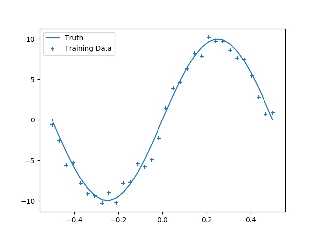
Construct Bayesian Neural Network
mutable struct VariationalLayer
    units
    activation
    prior_σ1
    prior_σ2
    prior_π1
    prior_π2
    Wμ
    bμ
    Wρ
    bρ
    init_σ
end

function VariationalLayer(units; activation=relu, prior_σ1=1.5, prior_σ2=0.1,
        prior_π1=0.5)
    init_σ = sqrt(
        prior_π1 * prior_σ1^2 + (1-prior_π1)*prior_σ2^2
    )
    VariationalLayer(units, activation, prior_σ1, prior_σ2, prior_π1, 1-prior_π1,
                        missing, missing, missing, missing, init_σ)
end

function kl_loss(vl, w, μ, σ)
    dist = ADCME.Normal(μ,σ)
    return sum(logpdf(dist, w)-logprior(vl, w))
end

function logprior(vl, w)
    dist1 = ADCME.Normal(constant(0.0), vl.prior_σ1)
    dist2 = ADCME.Normal(constant(0.0), vl.prior_σ2)
    log(vl.prior_π1*exp(logpdf(dist1, w)) + vl.prior_π2*exp(logpdf(dist2, w)))
end

function (vl::VariationalLayer)(x)
    x = constant(x)
    if ismissing(vl.bμ)
        vl.Wμ = get_variable(vl.init_σ*randn(size(x,2), vl.units))
        vl.Wρ = get_variable(zeros(size(x,2), vl.units))
        vl.bμ = get_variable(vl.init_σ*randn(1, vl.units))
        vl.bρ = get_variable(zeros(1, vl.units))
    end
    Wσ = softplus(vl.Wρ)
    W = vl.Wμ + Wσ.*normal(size(vl.Wμ)...)
    bσ = softplus(vl.bρ)
    b = vl.bμ + bσ.*normal(size(vl.bμ)...)
    loss = kl_loss(vl, W, vl.Wμ, Wσ) + kl_loss(vl, b, vl.bμ, bσ)
    out = vl.activation(x * W + b)
    return out, loss
end

function neg_log_likelihood(y_obs, y_pred, σ)
    y_obs = constant(y_obs)
    dist = ADCME.Normal(y_pred, σ)
    sum(-logpdf(dist, y_obs))
end

ipt = placeholder(X)
x, loss1 = VariationalLayer(20, activation=relu)(ipt)
x, loss2 = VariationalLayer(20, activation=relu)(x)
x, loss3 = VariationalLayer(1, activation=x->x)(x)

loss_lf = neg_log_likelihood(y, x, noise)
loss = loss1 + loss2 + loss3 + loss_lf
Optimization
We use an ADAM optimizer to optimize the loss function. In this case, quasi-Newton methods that are typically used for deterministic function optimization are not appropriate because the loss function essentially involves stochasticity.
Another caveat is that because the neural network may have many local minimum, we need to run the optimizer multiple times in order to obtain a good local minimum.
opt = AdamOptimizer(0.08).minimize(loss)
sess = Session(); init(sess)
@showprogress for i = 1:5000
    run(sess, opt)
end


X_test = reshape(LinRange(-1.5,1.5,32)|>Array, :, 1)
y_pred_list = []
@showprogress for i = 1:10000
    y_pred = run(sess, x, ipt=>X_test)
    push!(y_pred_list, y_pred)
end

y_preds = hcat(y_pred_list...)

y_mean = mean(y_preds, dims=2)[:]
y_std = std(y_preds, dims=2)[:]

close("all")
plot(X_test, y_mean)
scatter(X[:], y[:], marker="+")
fill_between(X_test[:], y_mean-2y_std, y_mean+2y_std, alpha=0.5)