Optimizers

ADCME provides a rich class of optimizers and acceleration techniques for conducting inverse modeling. The programming model also allows for easily extending ADCME with customer optimizers. In this section, we show how to take advantage of the built-in optimization library by showing how to solve an inverse problem–estimating the diffusivity coefficient of a Poisson equation from sparse observations–using different kinds of optimization techniques.

Solving an Inverse Problem using L-BFGS optimizer

Consider the Poisson equation in 2D:

\[\begin{aligned} \nabla \cdot (\kappa (x,y)\nabla u(x,y)) &= f(x) & (x,y) \in \Omega\\ u(x,y) &=0 & (x,y)\in \partial \Omega \end{aligned}\tag{1}\]

Here $\Omega$ is a L-shaped domain, which can be loaded using meshread.

\[f(x,y) = -\sin\left(20\pi y+\frac{\pi}{8}\right)\]

and the diffusivity coefficient $\kappa(x,y)$ is given by

\[\kappa(x,y) = 2+e^{10x} - (10y)^2\]

We can solve Equation 1 using a standard finite element method. Here, we use AdFem.jl to solve the PDE.

using AdFem
using ADCME
using PyPlot 

function kappa(x, y)
    return 2 + exp(10x) - (10y)^2
end

function f(x, y)
    return sin(2π*10y+π/8)
end

mmesh = Mesh(joinpath(PDATA, "twoholes_large.stl"))

Kappa = eval_f_on_gauss_pts(kappa, mmesh)
F = eval_f_on_gauss_pts(f, mmesh)
L = compute_fem_laplace_matrix1(Kappa, mmesh)
RHS = compute_fem_source_term1(F, mmesh)

bd = bcnode(mmesh)
L, RHS = impose_Dirichlet_boundary_conditions(L, RHS, bd, zeros(length(bd)))

SOL = L\RHS 
close("all")
figure(figsize = (10, 4))
subplot(121)
visualize_scalar_on_gauss_points(Kappa, mmesh)
title("\$\\kappa\$")
subplot(122)
visualize_scalar_on_fem_points(SOL, mmesh)
title("Solution")
savefig("optimizers_poisson.png")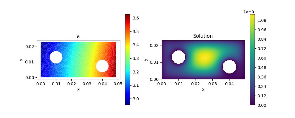

Now we approximate $\kappa(x,y)$ using a deep neural network (fc in ADCME). The script is nearly the same as the forward computation

using AdFem
using ADCME
using PyPlot 

function f(x, y)
    return sin(2π*10y+π/8)
end

mmesh = Mesh(joinpath(PDATA, "twoholes_large.stl"))

xy = gauss_nodes(mmesh)
Kappa = squeeze(fc(xy, [20, 20, 20, 1])) + 1.0
F = eval_f_on_gauss_pts(f, mmesh)
L = compute_fem_laplace_matrix1(Kappa, mmesh)
RHS = compute_fem_source_term1(F, mmesh)

bd = bcnode(mmesh)
L, RHS = impose_Dirichlet_boundary_conditions(L, RHS, bd, zeros(length(bd)))

sol = L\RHS 

We want to find a deep neural network such that sol and SOL match. We can train the neural network by minimizing a loss function.

loss = sum((sol - SOL)^2)*1e10

Here we multiply the loss function by 1e10 because the scale of SOL is $10^{-5}$. We want the initial value of loss to have a scale of $O(1)$.

We can minimize the loss function by

sess = Session(); init(sess)
losses = BFGS!(sess, loss)

We can visualize the result:

figure(figsize = (10, 4))
subplot(121)
semilogy(losses)
xlabel("Iterations"); ylabel("Loss")
subplot(122)
visualize_scalar_on_gauss_points(run(sess, Kappa), mmesh)
savefig("optimizer_bfgs.png")

We see that the estimated $\kappa(x,y)$ is quite similar to the reference one.

Use the optimizer from Optim.jl

We have used the built-in optimizer L-BFGS. What if we want to try out other options? Optimize! is an API that allows you to try out custom optimizers. For convenience, it also supports optimizers from the Optim.jl package.

Let's consider using BFGS to solve the above problem:

import Optim
sess = Session(); init(sess)
losses = Optimize!(sess, loss, optimizer = Optim.BFGS())

figure(figsize = (10, 4))
subplot(121)
semilogy(losses)
xlabel("Iterations"); ylabel("Loss")
subplot(122)
visualize_scalar_on_gauss_points(run(sess, Kappa), mmesh)
savefig("optimizer_bfgs2.png")

Unfortunately, it got stuck after several iterations.

Build Your Own Optimizer

Sometimes we might want to build our own optimizer. This can be done using Optimize!. To this end, we want to supply the function with the following arguments:

• sess: Session
• loss: Loss function to minimize
• optimizer: a keyword argument that specifies the optimizer function. The function takes f, fprime, and f_fprime (outputs both loss and gradients), initial value x0 as input. The output is redirected to the output of Optimize!.

Let us consider minimizing the Rosenbrock function using an optimizer from Ipopt

import Ipopt
x = Variable(rand(2))
loss = (1-x[1])^2 + 100(x[2]-x[1]^2)^2

function opt(f, g, fg, x0)
    prob = createProblem(2, -100ones(2), 100ones(2), 0, Float64[], Float64[], 0, 0,
                     f, (x,g)->nothing, (x,G)->g(G, x), (x, mode, rows, cols, values)->nothing, nothing)
    prob.x = x0 
    Ipopt.addOption(prob, "hessian_approximation", "limited-memory")
    status = Ipopt.solveProblem(prob)
    println(Ipopt.ApplicationReturnStatus[status])
    println(prob.x)
    Ipopt.freeProblem(prob)
    nothing
end

sess = Session(); init(sess)
Optimize!(sess, loss, optimizer = opt)