Distributed Scientific Machine Learning using MPI

Many large-scale scientific computing involves parallel computing. Among many parallel computing models, the MPI is one of the most popular models. In this section, we describe how ADCME can work with MPI for solving inverse modeling. Specifically, we describe how gradients can be back-propagated via MPI function calls.

MPI Support in ADCME

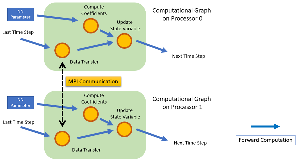
The ADCME solution to distributed computing for scientific machine learning is to provide a set of "data communication" nodes in the computational graph. Each machine (MPI processor) runs an identical computational graph. The computational nodes are executed independently on each processor, and the data communication nodes need to synchronize among different processors.

These data communication nodes are implemented using MPI APIs. They are not necessarily blocking operations, but because ADCME respects the data dependency of computation, they act like blocking operations and the child operators are executed only when data communication is finished. For example, in the following example,

b = mpi_op(a)
c = custom_op(b)

even though mpi_op and custom_op can overlap, ADCME still sequentially execute these two operations.

This blocking behavior simplifies the synchronization logic as well as the implementation of gradient back-propagation while harming little performance.

ADCME provides a set of commonly used MPI operators. See MPI Operators. Basically, they are

• mpi_init, mpi_finalize: Initialize and finalize MPI session.
• mpi_rank, mpi_size: Get the MPI rank and size.
• mpi_sum, mpi_bcast: Sum and broadcast tensors in different processors.
• mpi_send, mpi_recv: Send and receive operators.

The above two set of operators support automatic differentiation. They were implemented with MPI adjoint methods, which have existed in academia for decades.

This section shows how to configure MPI for distributed computing in ADCME.

Limitations

Despite that the provided mpi_* operations meet most needs, some sophisticated data communication operations may not be easily expressed using these APIs. For example, when solving the Poisson's equation on a uniform grid, we may decompose the domain into many squares, and two adjacent squares exchange data in each iteration. A sequence of mpi_send, mpi_recv will likely cause deadlock.

Just like when it is difficult to use automatic differentiation to implement a forward computation and its gradient back-propagation, we resort to custom operators, it is the same case for MPI. We can design a specialized custom operator for data communication. To resolve the deadlock problem, we found the asynchronous sending, followed by asynchronous receiving, and then followed by waiting, a very general and convenient way to implement custom operators.

Implementing Custom Operators using MPI

We can also make custom operators with MPI. Let us consider computing

\[f(\theta) = \sum_{i=1}^n f_i(\theta)\]

Each $f_i$ is a very expensive function so it makes sense to use MPI to split the jobs on different processors. To simplify the problem, we consider

\[f(\theta) = f_1(\theta) + f_2(\theta) + f_3(\theta) + f_4(\theta)\]

where $f_i(\theta) = \theta^{i-1}$.

Using the ADCME MPI API, we have the following code (test_simple.jl)

using ADCME

mpi_init()
θ = placeholder(ones(1))
fθ = mpi_bcast(θ)
l = fθ^mpi_rank()
L = sum(mpi_sum(l))
g = gradients(L, θ)
sess = Session(); init(sess)
L_ = run(sess, L, θ=>ones(1)*2.0)
g_ = run(sess, g, θ=>ones(1)*2.0)

if mpi_rank()==0
    @info  L_, g_ 
end
mpi_finalize()

We run the program with 4 processors

mpirun -n 4 julia test_simple.jl

We have the results:

[ Info: (15.0, [17.0])

Hybrid Programming

Each MPI processor can communicate data between processes, which do not share memory. Within each process, ADCME also allows for multi-threaded parallelism with a shared-memory model. For example, we can use OpenMP to accelerate matrix vector production. We can also use a threadpool per process to manage more complex and dynamic parallel tasks. However, the hybrid model brings challenges to communicate data using MPI. When we post MPI calls from different threads within the same process, we need to prevent data races and match the corresponding broadcast and collective operators. For example, without any guarantee on the ordering of concurrent MPI calls, we might incorrectly matched a send operator with a gather operator.

In ADCME, we adopt the dependency injection technique: we explicitly serialize the MPI calls by adding ghost dependencies. For example, in the following computational graph, originally, Operator 2 and Operator 3 are independent. In a concurrent computing environment, Rank 0 may execute Operator 2 first and then Operator 3, while Rank 1 executes Operator 3 first and then Operator 2. Then there is a mismatch of the MPI call (race condition): Operator 2 in Rank 0 coacts with Operator 3 in Rank 1, and Operator 3 in Rank 0 coacts with Operator 2 in Rank 1.

To resolve the data race issue, we can explicitly make Operator 3 depend on Operator 2. In this way, we can ensure that the MPI calls Operator 1, 2, and 3 are executed in order. Note this technique sacrifices some concurrency (Operator 2 and Operator 3 cannot be executed concurrently), but the concurrency of most non-MPI operators is still preserved.

Optimization

For solving inverse problems using distributed computing, an MPI-capable optimizer is required. The ADCME solution to distributed optimization is that the master machine holds, distributes and updates the optimizable variables. The gradients are calculated in the same device where the corresponding forward computation is done. Therefore, for a given serial optimizer, we can refactor it to a distributed one by letting worker nodes wait for instructions from the master node to compute either the objective function or the gradient.

This idea is implemented in the ADOPT.jl package, a customized version of Optim.jl. In ADCME, we provide a wrapper mpi_optimize.

In the following, we try to solve

\[1+\theta +\theta^2+\theta^3 = 2\]

using MPI-enabled LBFGS optimizer.

using ADCME
import Optim
mpi_init()
θ = placeholder(ones(1))
fθ = mpi_bcast(θ)
l = fθ^(mpi_rank()+1)
L = (sum(mpi_sum(l)) - 2.0)^2
g = gradients(L, θ)
sess = Session(); init(sess)

f = x->run(sess, L, θ=>x)
g! = (G, x)->(G[:] = run(sess, g, θ=>x))

result = mpi_optimize(f, g!, ones(1))
if mpi_rank()==0
    @info  result.minimizer, result.minimum
end

mpi_finalize()


### Reduce Sum

julia using ADCME

mpiinit() r = mpirank() a = constant(Float64.(Array(1:10) * r)) b = mpi_sum(a)

L = sum(b) g = gradients(L, a) sess = Session(); init(sess) v, G = run(sess, [b,g]) mpi_finalize()

### Broadcast

julia using ADCME

mpiinit() r = mpirank() a = constant(ones(10) * r) b = mpibcast(a, 3) L = sum(b^2) L = mpisum(L) g = gradients(L, a)

sess = Session(); init(sess) v, G = run(sess, [b, G]) mpi_finalize()

### Send and Receive

julia

mpiexec.exe -n 4 julia .\mpisum.jl

using ADCME

mpiinit() r = mpirank() a = constant(ones(10) * r) a = mpi_sendrecv(a, 0, 2)

L = sum(a^2) g = gradients(L, a)

sess = Session(); init(sess) v, G = run(sess, [a,g]) mpi_finalize()

[`mpi_sendrecv`](@ref) is a lightweight wrapper for [`mpi_send`](@ref) followed by [`mpi_recv`](@ref). Equivalently, we have

julia if r==2 global a a = mpisend(a, 0) end if r==0 global a a = mpirecv(a,2) end

## Solving the Heat Equation

In this section, we consider solving the Poisson equation 

$$\frac{\partial u(x,y)}{\partial t} =\kappa(x,y) \Delta u(x,y) \quad (x,y) \in [0,1]^2$$

We discretize the above PDE with an explicit finite difference scheme

$$\frac{u_{ij}^{n+1} - u^n_{ij}}{\Delta t} = \kappa_{ij} \frac{u_{i+1,j}^n + u_{i,j+1}^n + u_{i,j-1}^n + u_{i-1,j}^n - 4u_{ij}^n}{h^2} \tag{1}$$

To mitigate the computational and memory requirement, we use MPI APIs to implement a domain decomposition solver for the heat equation. The mesh is divided into $N\times M$ rectangle patches. We implemented two operation:

1. `heat_op`, which updates $u_{ij}^{n+1}$ using Equation 1 for a specific patch, with state variables $u_{ij}^n$ in the current rectangle patch and on the boundary (from adjacent patches). 

2. `data_exchange`, which is a data communication operator that sends the boundary data to adjacent patches and receives boundary data from other patches. 

![](https://github.com/ADCMEMarket/ADCMEImages/blob/master/ADCME/dataexchange.png?raw=true)

Then the time marching scheme can be implemented with the following code:

julia function heatupdateu(u, kv, f) r = mpi_rank() I = div(r, M) J = r%M

up_ = constant(zeros(m))
down_ = constant(zeros(m))
left_ = constant(zeros(n))
right_ = constant(zeros(n))


up = constant(zeros(m))
down = constant(zeros(m))
left = constant(zeros(n))
right = constant(zeros(n))

(I>0) && (up = u[1,:])
(I<N-1) && (down = u[end,:])
(J>0) && (left = u[:,1])
(J<M-1) && (right = u[:,end])

left_, right_, up_, down_ = data_exchange(left, right, up, down)

u = heat(u, kv, up_, down_, left_, right_, f, h, Δt)

end

An MPI-capable heat equation time integrator can be implemented with 

julia function heatsolver(u0, kv, f, NT=10) f = constant(f) function condition(i, uarr) i<=NT end function body(i, uarr) u = read(uarr, i) unew = heatupdateu(u, kv, f[i]) # op = tf.print(r, i) # unew = bind(unew, op) i+1, write(uarr, i+1, unew) end i = constant(1, dtype =Int32) uarr = TensorArray(NT+1) uarr = write(uarr, 1, u0) , u = whileloop(condition, body, [i, u_arr]) reshape(stack(u), (NT+1, n, m)) end

For example, we can implement the heat solver with diffusivity coefficient $K_0$ and initial condition $u_0$ with the following code:

julia K = placeholder(K0) a_ = mpibcast(K) sol = heatsolver(u0, K_, F, NT) ```