Optimal Transport

Optimal transport (OT) can be used to measure the "distance" between two probability distribution.

Discrete Wasserstein Distance

In this section, we introduce a novel approach for training a general model: SinkHorn Generative Networks (SGN). In this approach, a neural network is used to transform a sample from uniform distributions to a sample of targeted distribution. We train the neural network by minimizing the discrepancy between the targeted distribution and the desired distribution, which is described by optimal transport distance. Different from generative adversarial nets (GAN), we do not use a discriminator neural network to construct the discrepancy; instead, it is computed directly with efficient SinkHorn algorithm or net-flow solver. The minimization is conducted via a gradient-based optimizer, where the gradients are computed with reverse mode automatic differentiation.

To begin with, we first construct the sample x of the targeted distribution and the sample s from the desired distribution and compute the loss function with sinkhorn

using Revise
using ADCME
using PyPlot

reset_default_graph()
K = 64
z = placeholder(Float64, shape=[K, 10])
x = squeeze(ae(z, [20,20,20,1]))
s = placeholder(Float64, shape=[K])
M = abs(reshape(x, -1, 1) - reshape(s, 1, -1))
loss = sinkhorn(ones(K)/K, ones(K)/K, M, reg=0.1)

Example 1 In the first example, we assume the desired distribution is the standard Gaussian. We minimize the loss function with the Adam optimizer

opt = AdamOptimizer().minimize(loss)
sess = Session(); init(sess)
for i = 1:10000
    _, l = run(sess, [opt, loss], z=>rand(K, 10), s=>randn(K))
    @show i, l
end

The result is shown below

V = []
for k = 1:100
    push!(V,run(sess, x, z=>rand(K,10)))
end
V = vcat(V...)
hist(V, bins=50, density=true)
x0 = LinRange(-3.,3.,100)
plot(x0, (@. 1/sqrt(2π)*exp(-x0^2/2)), label="Reference")
xlabel("x")
ylabel("f(x)")
legend()

Example 2 In the first example, we assume the desired distribution is the positive part of the the standard Gaussian.

opt = AdamOptimizer().minimize(loss)
sess = Session(); init(sess)
for i = 1:10000
    _, l = run(sess, [opt, loss], z=>rand(K, 10), s=>abs.(randn(K)))
    @show i, l
end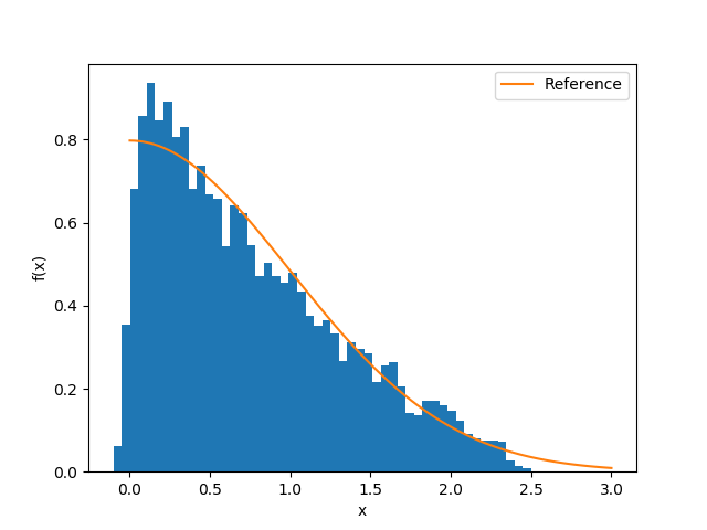

Dynamic Time Wrapping

Dynamic time wrapping is suitable for computing the distance of two time series. The idea is that we can shift the time series to obtain the "best" match while retaining the causality in time. This is best illustrated in the following figure

In ADCME, the distance is computed using dtw. As an example, given two time series

Sample = Float64[1,2,3,5,5,5,6]
Test = Float64[1,1,2,2,3,5]

The distance can be computed by

c, p = dtw(Sample, Test, true)

c is the distance and p is the path.

If we have 2000 time series A and 2000 time series B and we want to compute the total distance of the corresponding time series, we can use map function

A = constant(rand(2000,1000))
B = constant(rand(2000,1000))
distance = map(x->dtw(x[1],x[2],false)[1],[A,B], dtype=Float64)

distances is a 2000 length vector and gives us the pairwise distance for all time series.