Finite-difference Time-domain for Electromagnetics and Seismic Inversion

The finite-difference time-domain (FDTD) is a very conceptually and technically simple technique for full-wave simulation. It has been widely adopted in electromagnetics and geophysics. For example, the full-waveform inversion (FWI), which is arguably the most famous seismic inversion technique, is typically implemented with FDTD. It is also known as Yee scheme. Given its significance, in this section, we show how to implement FDTD in one-dimension using ADCME, and use the forward computation code to do inverse problems.

FDTD

To make the discussion clear and consistent throughout the session, we use notations from electromagnetics, $E$, the electric field, and $H$, the magnetic flux. In 1D, the Faraday's law and Ampere's law are simplified to

\[\begin{aligned} \mu \frac{\partial H}{\partial t} &= \frac{\partial E}{\partial x}\\ \epsilon \frac{\partial E}{\partial t} &= \frac{\partial H}{\partial x} \end{aligned}\]

We use the staggered grid shown in the following figure

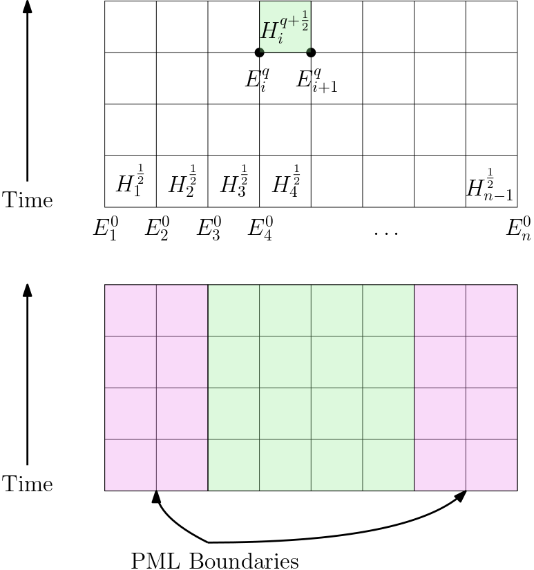
The superscript denotes time step, while the subscript denotes location index. The electric field $E_i^q$ is defined on the grid point, while the magnetic flux is defined in the cell center. The Yee algorithm alternatively updates $H$ and $E$ with

\[\begin{aligned} H_i^{q+\frac12} & = H_i^{q-\frac12} + \frac{\Delta t}{\mu\Delta x} (E^q_{i+1} - E^q_i)\\ E_i^{q+1} &= E_i^{q} + \frac{\Delta t}{\epsilon \Delta x}(H^{q+\frac12}_{i} - H^{q+\frac12}_{i-1}) \end{aligned}\]

When we simulate within a finite computational domain, we usually need to design a boundary condition that "absorbs" reflecting waves. This can be done with the so-called perfectly matched layer (PML) boundaries. In practice, we can pad the computational domain with extra grids (the magenta region in the figure above). See the next section for a detailed discussion.

In the case we want to add some source functions, there are typically two ways:

• Hardwiring source functions by setting $E_k^q=s_k^q$ for all $q$ and certain index $k$.
• Additive source functions. This is achieved by replacing the second equation with

\[E_i^{q+1} = E_i^{q} + \frac{\Delta t}{\epsilon \Delta x}(H^{q+\frac12}_{i} - H^{q+\frac12}_{i-1}) + \frac{\Delta t}{\epsilon} J_i^{q+\frac12}\]

Perfectly Matched Layer (PML)

Let us consider the plane wave $e^{i kx}$. In the infinite space, the plane wave will pass through the domain of interest and never get reflected back. However, in practice, computational domains are finite. If we impose a reflection boundary condition, the plane wave will get reflected. Even if we impose Dirichlet boundary conditions, some portions of reflection is still present. These reflections are not desirable for relevant applications. Therefore, we want to find a way for damping reflected waves away.

Let us consider the plane waves $e^{ikx}$. It's complex but we can always think of it as an analytical continuous of $sin(kx)$ in the complex space. Instead of looking at real $x$, we consider a complex $x$, and we have

\[e^{ik(\Re x + i\Im x)} = e^{ik\Re x - k\Im x}\]

Here is an important observation: if $\Im x = f(\Re x) >0$ for some increasing function $f(x)$, the magnitude of the wave $e^{ikx}$ along the line $\Re x + i f(\Re x)$ will decay exponentially. Thus, within a finite computational domain $[0,1]$, we can extend the governing equation beyond $[0,1]$ in the complex domain, with the path given by

\[\{ x + i f(x): x\in \mathbb{R}\}\]

Here $f(x) = 0$, $x\in (0,1)$, and

\[f'(x) = \frac{\sigma(x)}{k}, x>1\]

The case for $f(x)<0$ is similar.

The fundamental idea is that instead of looking at the governing equation in $[0,1]$, we extend it analytically into the complex space. For example, the transport equation

\[\frac{\partial u(x, t)}{\partial t} = \frac{\partial u(x, t)}{\partial x}\]

becomes

\[\frac{\partial \tilde u(z, t)}{\partial t} = \frac{\partial \tilde u(z, t)}{\partial z}, z\in \mathbb{C}\]

Then the question is: what is the governing equation for $\bar u(x, t) = \tilde u(x+i f(x), t)$?

To simplify our notation, we omit $t$ here because it is unrelated to the complex domain. We denote $z = x + i f(x)$ and

\[\Re \tilde u = u_1, \Im \tilde u = u_2\]

Then we have

\[\begin{aligned} \frac{\partial \bar u(x)}{\partial x} &= \frac{\partial \tilde u(x+i f(x))}{\partial x}\\ &= \frac{\partial (u_1(x+i f(x)) + i u_2(x+i f(x)))}{\partial x}\\ &= \frac{\partial (u_1(x+i f(x))}{\partial x} + i \frac{\partial u_2(x+i f(x)))}{\partial x} \\ &= \frac{\partial u_1}{\partial x} + i \frac{\partial u_2}{\partial x} + i \frac{\partial u_1}{\partial x} \frac{\partial f}{\partial x} - \frac{\partial u_2}{\partial x}\frac{\partial f}{\partial x} \end{aligned}\]

Note from complex analysis,

\[\frac{\partial \tilde u(z)}{\partial z} = \frac{\partial u_1}{\partial x} + i \frac{\partial u_2}{\partial x}\]

We have

\[\frac{\partial \bar u(x)}{\partial x} =\left(1 + i\frac{\partial f}{\partial x} \right) \frac{\partial \tilde u}{\partial z}\tag{1}\]

Now let us consider the Faraday's law

\[\mu \frac{\partial H}{\partial t} = \frac{\partial E}{\partial x}\tag{2}\]

We consider the plane wave $H = e^{-ikx}$, which we want to damp outside the computational domain. First we extend Equation 2 to the complex domain and plug $H$ to the equation (note $\frac{\partial H}{\partial t} = \frac{\partial \bar H}{\partial t}$)

\[-i\mu k \bar H = \frac{\partial \tilde E}{\partial z}\]

Using Equation 1, we have

\[-i \mu k \bar H+ \mu \sigma_x(x) \bar H= \frac{\partial \bar E}{\partial x}\]

Converting back to the time domain, we have

\[\mu\frac{\partial \bar H}{\partial t} = \frac{\partial \bar E}{\partial x} - \mu \sigma_x(x) \bar H\]

Likewise, we have

\[\epsilon\frac{\partial \bar H}{\partial t} = \frac{\partial \bar E}{\partial x} - \epsilon \sigma_x(x) \bar H\]

Note that the two above equations are exactly the original equations within the domain $[0,1]$.

Numerical Experiment: Forward Computation

Let us consider a 1D wave equation

\[\frac{\partial^2 u}{\partial t^2} = c^2 \frac{\partial^2 u}{\partial x^2}\]

which is equivalent to

\[\begin{aligned} \frac{\partial u}{\partial t} &= c \frac{\partial v}{\partial x}\\ \frac{\partial v}{\partial t} &= c \frac{\partial u}{\partial x} \end{aligned}\]

This set of equations is related to Faraday's law and Ampere's law via

\[E = v, H = u, \epsilon = \frac1c, \mu = \frac1c\]

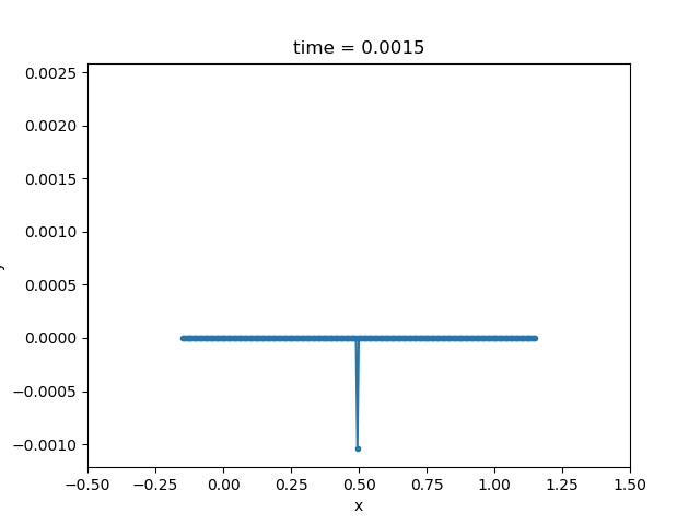
We use a hardwiring source at the center of the computational domain $[0,1]$. The source function is shown in the left panel. The evolution of $u$ is shown in the right panel.

|Source Function|Evolution of $u$| |–|–| |||

using ADCME
using PyPlot 
using ADCMEKit 

n = 200
pml = 30
C = 100.0
NT = 1000
Δt = 1.5/NT 
x0 = LinRange(0, 1, n+1)
h = 1/n 
xE = Array((0:n+2pml)*h .- pml*h)
xH = (xE[2:end]+xE[1:end-1])/2 
N = n + 2pml + 1

σE = zeros(N)
for i = 1:pml
    d = i*h
    σE[pml + n + 1 + i] = C* (d/(pml*h))^3
    σE[pml+1-i] = C* (d/(pml*h))^3
end

σH = zeros(N-1)
for i = 1:pml 
    d = (i-1/2)*h 
    σH[pml + n + i] = C* (d/(pml*h))^3
    σH[pml+1-i] = C* (d/(pml*h))^3
end

function ricker(dt = 0.002, f0 = 3.0)
    nw = 2/(f0*dt)
    nc = floor(Int, nw/2)
    t = dt*collect(-nc:1:nc)
    b = (π*f0*t).^2
    w = @. (1 - 2b)*exp(-b)
end
R = ricker()
if length(R)<NT+1
    R = [R;zeros(NT+1-length(R))]
end

R_ = constant(R)

# cH = constant(ones(N-1))
cH = ones(length(xH)) * 1.5
cE = (cH[1:end-1]+cH[2:end])/2
Z = zeros(N)
Z[N÷2] = 1.0
Z = Z[2:end-1]

function condition(i, E_arr, H_arr)
    i<=NT+1
end

function body(i, E_arr, H_arr)
    E = read(E_arr, i-1)
    H = read(H_arr, i-1)
    ΔH = cH * (E[2:end]-E[1:end-1])/h - σH*H
    H += ΔH * Δt
    ΔE = cE * (H[2:end]-H[1:end-1])/h - σE[2:end-1]*E[2:end-1] #+ R_[i] * Z
    E = scatter_add(E, 2:N-1, ΔE * Δt)
    E = scatter_update(E, N÷2, R_[i])
    i+1, write(E_arr, i, E), write(H_arr, i, H)
end

E_arr = TensorArray(NT+1)
H_arr = TensorArray(NT+1)

E0 = zeros(N)
E0[N÷2] = R[1]
E_arr = write(E_arr, 1, E0)
H_arr = write(H_arr, 1, zeros(N-1))

i = constant(2, dtype = Int32)

_, E, H = while_loop(condition, body, [i, E_arr, H_arr])

E = stack(E)
H = stack(H)

sess = Session(); init(sess)
E_, H_ = run(sess, [E, H])


pl, = plot([], [], ".-")
xlim(-0.5,1.5)
ylim(minimum(E_), maximum(E_))
xlabel("x")
ylabel("y")
t = title("time = 0.0000")
function update(i)
    t.set_text("time = $(round(i*Δt, digits=4))")
    pl.set_data([xE E_[i,:]]'|>Array)
end 
p = animate(update, 1:10:NT+1)
# saveanim(p, "fdtd.gif")

Numerical Experiment

Let us consider inverting for a constant $c_H$. The following code is mainly a copy and paste from the above code. The optimization converges within a few iterations.

using ADCME
using PyPlot 
using ADCMEKit 

n = 200
pml = 30
C = 100.0
NT = 1000
Δt = 1.5/NT 
x0 = LinRange(0, 1, n+1)
h = 1/n 
xE = Array((0:n+2pml)*h .- pml*h)
xH = (xE[2:end]+xE[1:end-1])/2 
N = n + 2pml + 1

σE = zeros(N)
for i = 1:pml
    d = i*h
    σE[pml + n + 1 + i] = C* (d/(pml*h))^3
    σE[pml+1-i] = C* (d/(pml*h))^3
end

σH = zeros(N-1)
for i = 1:pml 
    d = (i-1/2)*h 
    σH[pml + n + i] = C* (d/(pml*h))^3
    σH[pml+1-i] = C* (d/(pml*h))^3
end

function ricker(dt = 0.002, f0 = 3.0)
    nw = 2/(f0*dt)
    nc = floor(Int, nw/2)
    t = dt*collect(-nc:1:nc)
    b = (π*f0*t).^2
    w = @. (1 - 2b)*exp(-b)
end
R = ricker()
if length(R)<NT+1
    R = [R;zeros(NT+1-length(R))]
end

R_ = constant(R)

# cH = constant(ones(N-1))
# cH = Variable(ones(length(cH)))
b = softplus(Variable(1.0))
cH = ones(length(xH)) * b
cE = (cH[1:end-1]+cH[2:end])/2
Z = zeros(N)
Z[N÷2] = 1.0
Z = Z[2:end-1]

function condition(i, E_arr, H_arr)
    i<=NT+1
end

function body(i, E_arr, H_arr)
    E = read(E_arr, i-1)
    H = read(H_arr, i-1)
    ΔH = cH * (E[2:end]-E[1:end-1])/h - σH*H
    H += ΔH * Δt
    ΔE = cE * (H[2:end]-H[1:end-1])/h - σE[2:end-1]*E[2:end-1] #+ R_[i] * Z
    E = scatter_add(E, 2:N-1, ΔE * Δt)
    E = scatter_update(E, N÷2, R_[i])
    i+1, write(E_arr, i, E), write(H_arr, i, H)
end

E_arr = TensorArray(NT+1)
H_arr = TensorArray(NT+1)

E0 = zeros(N)
E0[N÷2] = R[1]
# v0[N÷2] = 1.0
E_arr = write(E_arr, 1, E0)
H_arr = write(H_arr, 1, zeros(N-1))

i = constant(2, dtype = Int32)

_, E, H = while_loop(condition, body, [i, E_arr, H_arr])

E = stack(E); E = set_shape(E, (NT+1, N))
H = stack(H)

receivers = [pml+1:pml+10; N-pml-9:N-pml]
loss = sum((E[:,receivers] - E_[:,receivers])^2)
sess = Session(); init(sess)
BFGS!(sess, loss)