Direct Methods for Sparse Matrices
Usage
The direct methods for sparse matrix solutions feature a matrix factorization for solving a set of equations. This procedure is call factorization or decomposition. We can also support factorization or decomposition via shared memory across kernels. The design is to store the factorized matrix in the C++ memory and pass an identifying code (an integer) to the solution operators. Here is how you solve $Ax_i = b_i$ for a list of $(x_i, b_i)$
Step 1: Factorization
A_factorized = factorize(A)Step2: Solve
x1 = A_factorized\b1
x2 = A_factorized\b2
......
Compared to A\b, the factorize-then-solve approach is more efficient, especially when you have to solve a lot of equations.
Control Flow Safety
The factorize-then-solve method is also control flow safe. That is, we can safely use it in the control flow and gradient backpropagation is correct. For example, if the matrix $A$ keeps unchanged throught the loop, we might want to factorize $A$ first and then use the factorized $A$ to solve equations repeatly. To verify the control flow safety, consider the following code, where in the loop we have
\[u_{i+1} = A^{-1}(u_i + r), i=1,2,\ldots\]
using ADCME
using SparseArrays
using ADCMEKit
function while_loop_simulation(vv, rhs, ns = 10)
A = SparseTensor(ii, jj, vv, 10, 10) + spdiag(10)*100.
Afac = factorize(A)
ta = TensorArray(ns)
i = constant(2, dtype=Int32)
ta = write(ta, 1, ones(10))
function condition(i, ta)
i<= ns
end
function body(i, ta)
u = read(ta, i-1)
res = Afac\(u + rhs)
# res = u
ta = write(ta, i, res)
i+1, ta
end
_, out = while_loop(condition, body, [i, ta])
sum(stack(out)^2)
end
sess = Session(); init(sess)
A = sprand(10, 10, 0.8)
ii, jj, vv = find(constant(A))
k = length(vv)
# Test 1: autodiff through A
pl = placeholder(rand(k))
res = while_loop_simulation(pl, rhs , 100)
gradview(sess, pl, res, rand(k))
# Test 2: autodiff through rhs
pl = placeholder(rand(10))
res = while_loop_simulation(vv, pl , 100)
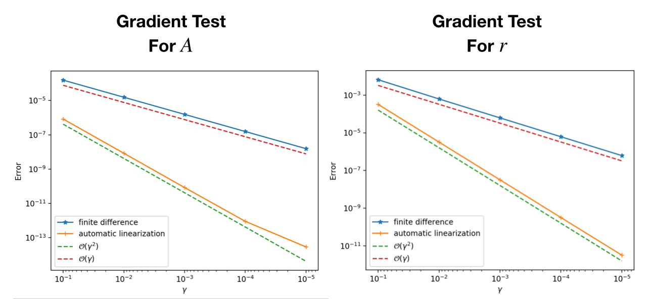
gradview(sess, pl, res, rand(10))We have the following convergence plot