Radial Basis Functions
The principle of radial basis functions (RBF) is to use linear combination of radial basis functions to approximate a function. The radial basis functions are usually global functions in the sense that its support spans over the entire domain. This property lends adaptivity and regularization to the RBF function form: unlike local basis functions such as piecewise linear functions, RBF usually does not suffer from local anomalies and produces a smoother approximation.
The mathematical formulation of RBFs on a 2D domain is as follows
\[f(x, y) = \sum_{i=1}^N c_i \phi(r; \epsilon_i) + d_0 + d_1 x + d_2 y\]
Here $r = \sqrt{|x-x_i|^2 + |y-y_i|^2}$. $\{x_i, y_i\}_{i=1}^N$ are called centers of the RBF, $c_i$ is the coefficient, $d_0+d_1x+d_2y$ is an additional affine term, and $\phi$ is a radial basis function parametrized by $\epsilon_i$. Four common radial basis functions are as follows (all are supported by ADCME)
- Gaussian
\[\phi(r; \epsilon) = e^{-(\epsilon r)^2}\]
- Multiquadric
\[\phi(r; \epsilon) = \sqrt{1+(\epsilon r)^2}\]
- Inverse quadratic
\[\phi(r; \epsilon) = \frac{1}{1+(\epsilon r)^2}\]
- Inverse multiquadric
\[\phi(r; \epsilon) = \frac{1}{\sqrt{1+(\epsilon r)^2}}\]
In ADCME, we allow $(x_i, y_i)$, $\epsilon_i$, $d_i$ and $c_i$ to be trainable (of course, users can allow only a subset to be trainable). This is done via RBF2D function. As an example, we consider using radial basis function to approximate
\[y = 1 + \frac{y^2}{1+x^2}\]
on the domain $[0,1]^2$. We use the following function to visualize the result
using PyPlot
n = 20
h = 1/n
x = Float64[]; y = Float64[]
for i = 1:n+1
for j = 1:n+1
push!(x, (i-1)*h)
push!(y, (j-1)*h)
end
end
close("all")
f = run(sess, rbf(x, y))
g = (@. 1+y^2/(1+x^2))
figure()
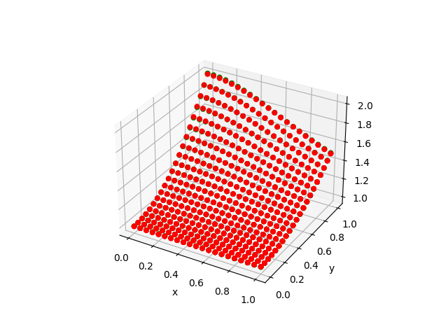
scatter3D(x, y, f, color="r")
scatter3D(x, y, g, color="g")
xlabel("x")
ylabel("y")
savefig("compare.png")
figure()
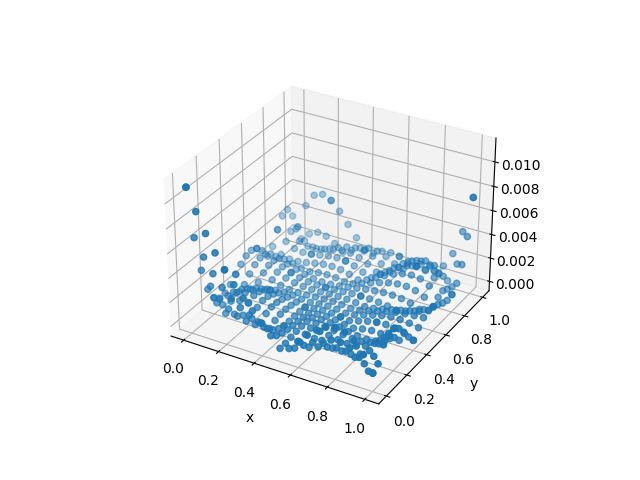
scatter3D(x, y, abs.(f-g))
xlabel("x")
ylabel("y")
savefig("diff.png")We consider several cases:
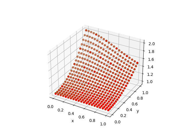
- Only $c_i$ is trainable
using ADCME

# use centers on a uniform grid
n = 5
h = 1/n
xc = Float64[]; yc = Float64[]
for i = 1:n+1
    for j = 1:n+1
        push!(xc, (i-1)*h)
        push!(yc, (j-1)*h)
    end
end

# by default, c is initialized to Variable(ones(...))
# eps is initialized to ones(...) and no linear terms are used
rbf = RBF2D(xc, yc)

x = rand(100); y = rand(100)
f = @. 1+y^2/(1+x^2)

fv = rbf(x, y)
loss = sum((f-fv)^2)

sess = Session(); init(sess)
BFGS!(sess, loss)| Approximation | Difference |
|---|---|
 |  |
- Only $c_i$ is trainable + Additional Linear Term
Here we need to specify d=Variable(zeros(3)) to tell ADCME we want both the constant and linear terms. If d=Variable(zeros(1)), only the constant term will be present.
using ADCME

# use centers on a uniform grid
n = 5
h = 1/n
xc = Float64[]; yc = Float64[]
for i = 1:n+1
    for j = 1:n+1
        push!(xc, (i-1)*h)
        push!(yc, (j-1)*h)
    end
end

# by default, c is initialized to Variable(ones(...))
# eps is initialized to ones(...) and no linear terms are used
rbf = RBF2D(xc, yc; d = Variable(zeros(3)))

x = rand(100); y = rand(100)
f = @. 1+y^2/(1+x^2)

fv = rbf(x, y)
loss = sum((f-fv)^2)

sess = Session(); init(sess)
BFGS!(sess, loss)| Approximation | Difference |
|---|---|
 |  |
- Free every trainable variables
xc = Variable(rand(25))
yc = Variable(rand(25))
d = Variable(zeros(3))
e = Variable(ones(25))

# by default, c is initialized to Variable(ones(...))
# eps is initialized to ones(...) and no linear terms are used
rbf = RBF2D(xc, yc; eps = e, d = d)

x = rand(100); y = rand(100)
f = @. 1+y^2/(1+x^2)

fv = rbf(x, y)
loss = sum((f-fv)^2)

sess = Session(); init(sess)
BFGS!(sess, loss)
We see we get much better result by freeing up all variables.
| Approximation | Difference |
|---|---|
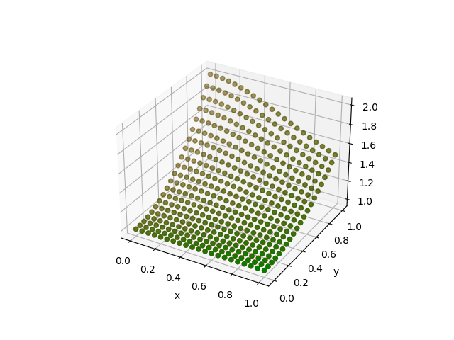 |  |
3D Radial Basis Function
ADCME also provides RBFs on a 3D domain. The usage of RBF3D is similar to RBF2D.
xc, yc, zc, c = rand(50), rand(50), rand(50), rand(50)
d = rand(4)
e = rand(50)
rbf = RBF3D(xc, yc, zc; c = c, d = d, eps = e)

x, y, z = rand(10), rand(10), rand(10)
v = rbf(x,y,z)

sess = Session()
run(sess, v)
Here xc, yc, and zc are the centers; e and d are hyper-parameters for radial basis functions (see API documentation for RBF3D). These parameter are trainable, e.g., we elect to train xc, yc, zc and e, and set $d=0$ (no linear affine term)
xc, yc, zc, c = Variable(rand(50)), Variable(rand(50)), Variable(rand(50)), Variable(rand(50))
e = Variable(rand(50))
rbf = RBF3D(xc, yc, zc; c = c, eps = e)

# ... (details ommited)

v = rbf(x, y, z)
loss = sum((v-vobs)^2)
sess = Session(); init(sess)
BFGS!(sess, loss)