Numerical Scheme in ADCME: Finite Difference Example
ADCME provides convenient tools to implement numerical schemes. In this tutorial, we will implement a finite difference program and conduct inverse modeling. In the first part, we consider a toy example of estimating parameters in a partial differential equation. In the second part, we showcase a real world application of ADCME to geophysical inversion.
Estimating a scalar unknown in the PDE
Consider the following partial differential equation
\[-bu''(x)+u(x)=f(x)\quad x\in[0,1], u(0)=u(1)=0\]
where
\[f(x) = 8 + 4x - 4x^2\]
Assume that we have observed $u(0.5)=1$, we want to estimate $b$. The true value in this case should be $b=1$. We can discretize the system using finite difference method, and the resultant linear system will be
\[(bA+I)\mathbf{u} = \mathbf{f}\]
where
\[A = \begin{bmatrix} \frac{2}{h^2} & -\frac{1}{h^2} & \dots & 0\\ -\frac{1}{h^2} & \frac{2}{h^2} & \dots & 0\\ \dots \\ 0 & 0 & \dots & \frac{2}{h^2} \end{bmatrix}, \quad \mathbf{u} = \begin{bmatrix} u_2\\ u_3\\ \vdots\\ u_{n} \end{bmatrix}, \quad \mathbf{f} = \begin{bmatrix} f(x_2)\\ f(x_3)\\ \vdots\\ f(x_{n}) \end{bmatrix}\]
The idea for implementing the inverse modeling method in ADCME is that we make the unknown $b$ a Variable and then solve the forward problem pretending $b$ is known. The following code snippet shows the implementation
using LinearAlgebra
using ADCME             # (1)

n = 101 # number of grid nodes in [0,1]
h = 1/(n-1)
x = LinRange(0,1,n)[2:end-1]       # (2)

b = Variable(10.0) # we use Variable keyword to mark the unknowns    # (3)
A = diagm(0=>2/h^2*ones(n-2), -1=>-1/h^2*ones(n-3), 1=>-1/h^2*ones(n-3))
B = b*A + I  # I stands for the identity matrix
f = @. 4*(2 + x - x^2)
u = B\f # solve the equation using built-in linear solver
ue = u[div(n+1,2)] # extract values at x=0.5								# (4)

loss = (ue-1.0)^2    # (5)

# Optimization
sess = Session(); init(sess) # (6)
BFGS!(sess, loss)			# (7)

println("Estimated b = ", run(sess, b))
The expected output is
Estimated b = 0.9995582304494237The detailed explaination is as follow: (1) The first two lines load necessary packages; (2) We split the interval $[0,1]$ into $100$ equal length subintervals; (3) Since $b$ is unknown and needs to be updated during optimization, we mark it as trainable using the Variable keyword; (4) Solve the linear system and extract the value at $x=0.5$. here I stands for the identity matrix and @. denotes element-wise operation. They are Julia-style syntax but are also compatible with tensors by overloading; (5) Formulate the loss function; (6) Create and initialize a TensorFlow session, which analyzes the computational graph and initializes the tensor values; (7) Finally, we trigger the optimization by invoking BFGS!, which wraps the L-BFGS-B algorithm.
ADSeismic.jl: A General Approach to Seismic Inversion
ADSeismic is a software package for solving seismic inversion problems, such as velocity model estimation, rupture imaging, earthquake location, and source time function retrieval. The governing equation for the acoustic wave equation is
$ \frac{\partial^2 u}{\partial t^2} = \nabla\cdot(c^2 \nabla u) + f$
where $u$ is displacement, $f$ is the source term, and $c$ is the spatially varying acoustic velocity. The inversion parameters of interest are $c$ or $f$. The governing equation for the elastic wave equation is
\[\begin{aligned} \rho \frac{\partial v_i}{\partial t} &= \sigma_{ij, j} + \rho f_i \\ \frac{\partial \sigma_{ij}}{\partial t} &= \lambda v_{k,k} + \mu(v_{i,j} + v_{j,i}) \end{aligned}\]
where $v$ is velocity, $\sigma$ is stress tensor, $\rho$ is density, and $\lambda$ and $\mu$ are the Lam\'e's constants. The inversion parameters in the elastic wave equation case are $\lambda$, $\mu$, $\rho$ or $f$.
The idea is to substitute the unknowns such as the $c$ and $f$ using mutable tensors (with the Variable keyword) and implement the finite difference method. The implementation detail is beyond the scope of this tutorial. Basically, when explicit schemes are used, the finite difference scheme can be expressed by a computational graph as follows, where $U$ is the discretization of $u$, $A(\theta)$ is the fintie difference coefficient matrix and $\theta$ is the unknown (in this case, the entries in the coefficient matrix depends on $\theta$ ). The loss function is formulated by matching the predicted wavefield $U_i$ and the observed wavefield $U_i^{\mathrm{obs}}$.
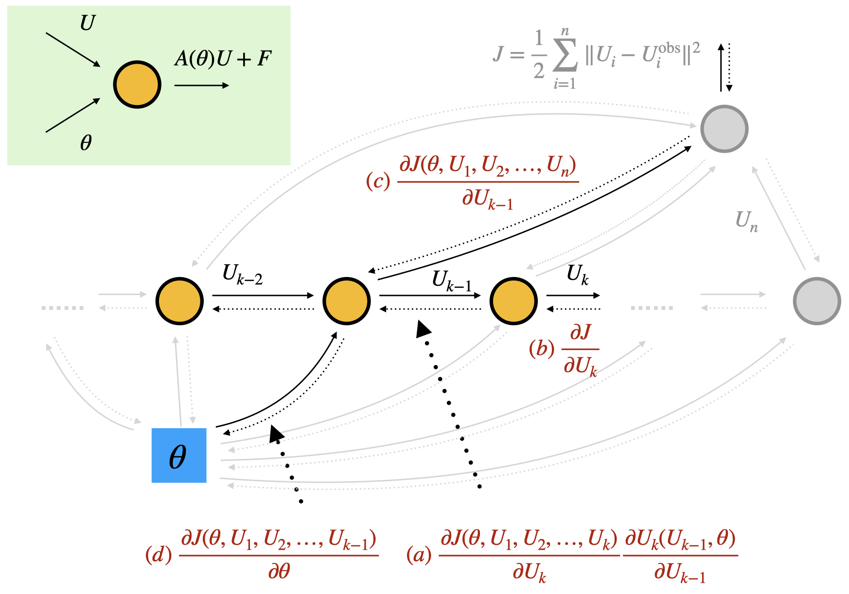
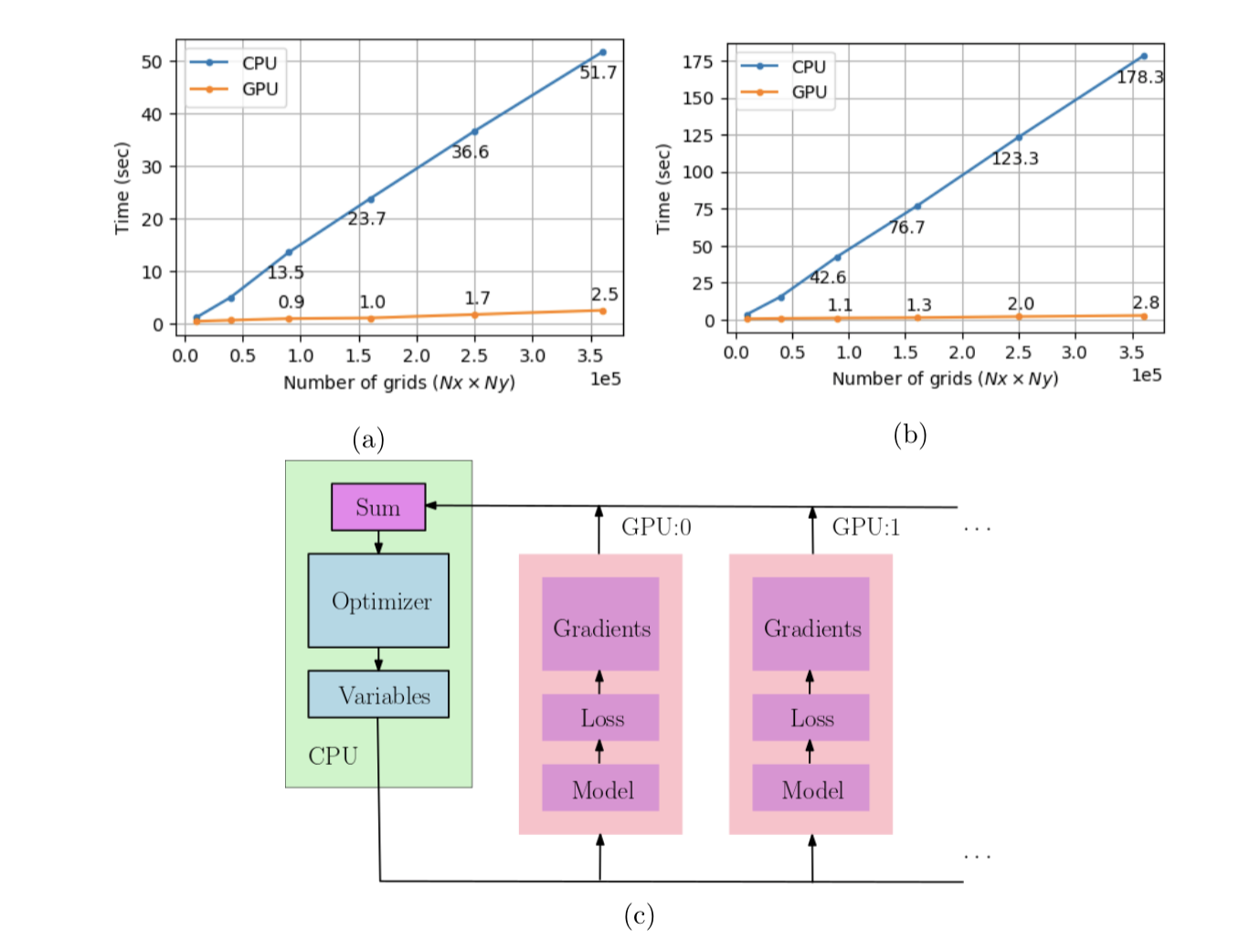
The unknown $\theta$ is sought by solving a minimization problem using L-BFGS-B, using gradients computed in AD. Besides the simplification of implementation, a direct benefit of implementing the numerical in ADCME is that we can leverage multi-GPU computing resources. We distribute the loss function for each scenario (in practice, we can collect many $\{U_i^{\mathbf{obs}}\}$ corresponding to different source functions $f$) onto different GPUs and compute the gradients separately. Using this strategy, we can achieve more than 20 times and 60 times acceleration for acoustic and elastic wave equations respectively.
Here we show a case in locating the centroid of an earthquake. The red star denotes the location where the earthquake happens and the triangles denote the seismic stations. The subsurface constitutes layers of different properties (the values of $c$ are different), affecting the propagation of the seismic waves.
| Source/Receiver Location | Forward Simulation |
|---|---|
 |  |
By running the optimization problem by specifying the earthquake location as Variable [delta], we can locate the centroid of an earthquake. The result is amazingly good. It is worth noting that it requires substantial effort to implement the traditional adjoint-state solver for this problem (e.g., it takes time to manually deriving and implementing the gradients). However, in view of ADCME, the inversion functionality is merely a by-product of the forward simulation codes, which can be reused in many other inversion problems.
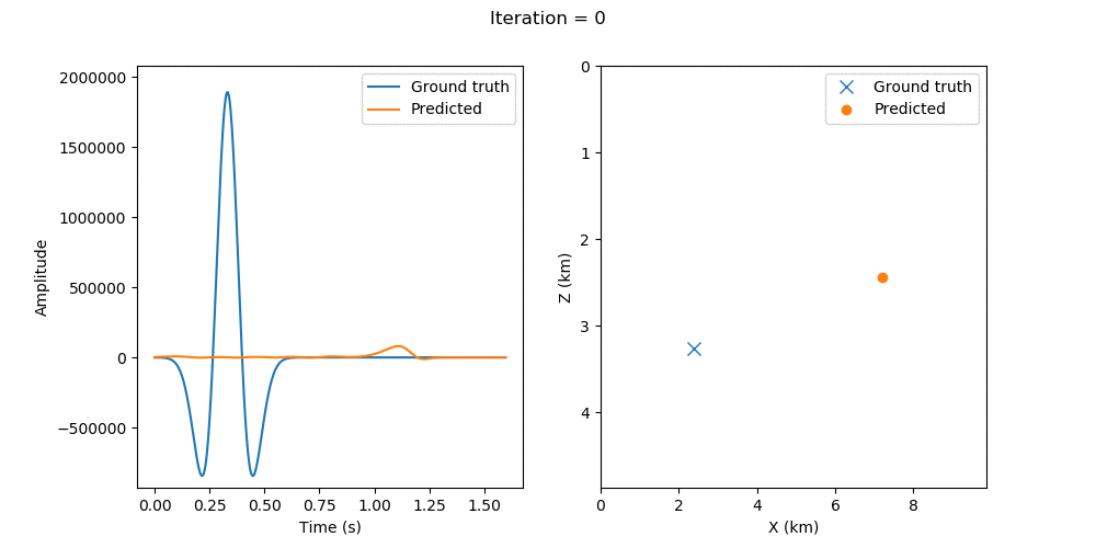
- deltaMathematically, $f(t, \mathbf{x})$ is a Delta function in $\mathbf{x}$; to make the inversion problem continuous, we use $f_{\theta}(t, \mathbf{x}) = g(t) \frac{1}{2\pi\sigma^2}\exp(-\frac{\|\mathbf{x}-\theta\|^2}{2\sigma^2})$ to approximate $f(t, \mathbf{x})$; here $\theta\in\mathbb{R}^2$ and $g(t)$ are unknown.