Advanced: Automatic Differentiation for Implicit Operators
An explicit operator is an operator directly supplied by the AD library while an implicit operator is an operator whose outputs must be computed using compositions of functions that may not be differentiable, or involving iterative algorithms. For example, $y = \texttt{sigmoid}(x)$ is an implicit operator while $x = \texttt{sigmoid}(y)$ is an implicit operator if the library does not provide $\texttt{sigmoid}^{-1}$, where $x$ is the input and $y$ is the output.
Implicit operators are everywhere in scientific computing, from implicit numerical schemes to iterative algorithms. How to incooperate implicit operators into a differentiable programming framework is the true challenge in AD. AD is not the panacea to all inverse modeling problems; it must be augmented with abilities to tackle implicit operators to be real useful for a large variety of real-world applications.
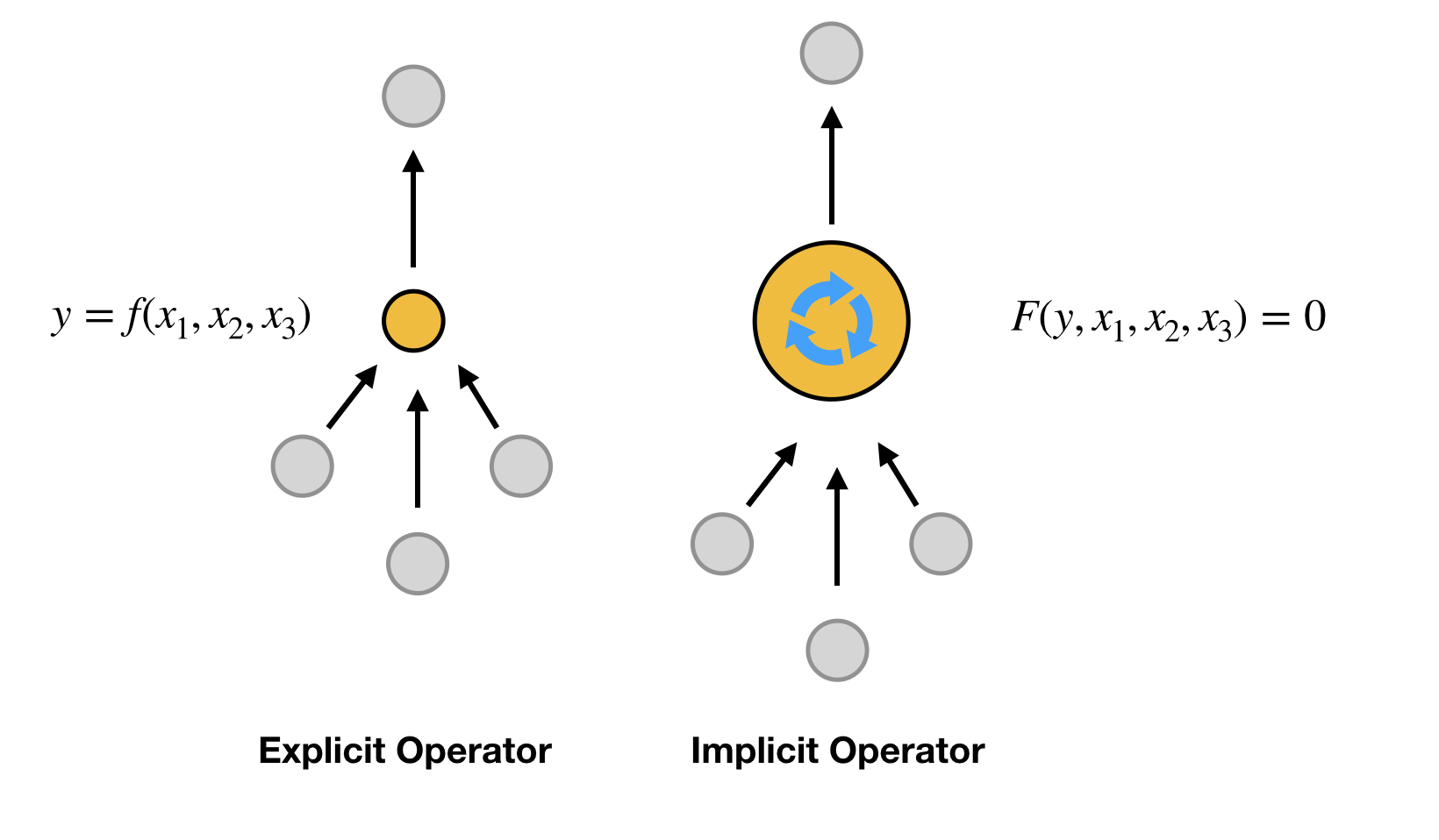
Roughly speaking, there are four types of operators in the computational graph, depending on whether it is linear or nonlinear and whether it is explicit or implicit. Let $A$ be a matrix, $f$ be a nonlinear function, $F$ be a bivariate nonlinear function, and it is hard to express $y$ analytically as a function of $x$ in $F(x,y)=0$.
| Operator | Linear | Nonlinear |
|---|---|---|
| Explicit | $y = Ax$ | $y = f(x)$ |
| Implicit | $Ay = x$ | $F(x, y)=0$ |
It is straightforward to apply AD to explicit operators, provided that the AD library supports the corresponding operators $A$ and $f$ (which usually do). In this tutorial, we focus on the implicit operators.
Implicit Function Theorem
We change our notation for clarity in this section. Let $L_h$ be a error functional, $F_h$ be the corresponding nonlinear implicit operator, $\theta$ is all the input to this operator and $u_h$ is all the output of this node.
\[\begin{aligned} \min_{\theta}&\; L_h(u_h) \\ \mathrm{s.t.}&\;\; F_h(\theta, u_h) = 0 \end{aligned}\]
Assume in the forward computation, we solve for $u_h=G_h(\theta)$ in $F_h(\theta, u_h)=0$, and then
\[\tilde L_h(\theta) = L_h(G_h(\theta))\]
Applying the implicit function theorem
\[\begin{aligned} & \frac{{\partial {F_h(\theta, u_h)}}}{{\partial \theta }} + {\frac{{\partial {F_h(\theta, u_h)}}}{{\partial {u_h}}}} \frac{\partial G_h(\theta)}{\partial \theta} = 0 \qquad \Rightarrow \\[4pt] & \frac{\partial G_h(\theta)}{\partial \theta} = -\Big( \frac{{\partial {F_h(\theta, u_h)}}}{{\partial {u_h}}} \Big)^{ - 1} \frac{{\partial {F_h(\theta, u_h)}}}{{\partial \theta }} \end{aligned}\]
therefore we have
\[\begin{aligned} \frac{{\partial {{\tilde L}_h}(\theta )}}{{\partial \theta }} &= \frac{\partial {{ L}_h}(u_h )}{\partial u_h}\frac{\partial G_h(\theta)}{\partial \theta} \\ &= - \frac{{\partial {L_h}({u_h})}}{{\partial {u_h}}} \; \Big( {\frac{{\partial {F_h(\theta, u_h)}}}{{\partial {u_h}}}\Big|_{u_h = {G_h}(\theta )}} \Big)^{ - 1} \; \frac{{\partial {F_h(\theta, u_h)}}}{{\partial \theta }}\Big|_{u_h = {G_h}(\theta )} \end{aligned}\]
This is the desired gradient. For efficiency, the computation strategy is crucial. We can either evaluate from left to right or from right to left. The correct approach is to compute from left to right. A detailed justification of this computational order is beyond the scope of this tutorial. Instead, we simply list the steps for calculating the gradients
Step 1: Calculate $w$ by solving a linear system (never invert the matrix!)
\[w^T = \underbrace{\frac{{\partial {L_h}({u_h})}}{{\partial {u_h}}\rule[-9pt]{1pt}{0pt}}}_{1\times N} \;\; \underbrace{\Big( {\frac{{\partial {F_h}}}{{\partial {u_h}}}\Big|_{u_h = {G_h}(\theta )}} \Big)^{ - 1}}_{N\times N}\]
Step 2: Calculate the gradient by automatic differentiation
\[w^T\;\underbrace{\frac{{\partial {F_h}}}{{\partial \theta }}\Big|_{u_h = {G_h}(\theta )}}_{N\times p} = \frac{\partial (w^T\; {F_h}(\theta, u_h))}{\partial \theta }\Bigg|_{u_h = {G_h}(\theta )}\]
This step can be done using independent, which stops back-propagating the gradients for its argument.
l  = L(u)
r  = F(theta, u)
g  = gradients(l, u)
x  = dF'\g
x  = independent(x)
dL = -gradients(sum(r*x), theta)
Despite the complex nature of this approach, it is quite powerful and efficient in treating implicit operators. To make it more clear, we consider a simpler special case below: the linear implicit operator.
Special Case: Linear Implicit Operator
The linear implicit operator can be viewed as a special case of the nonlinear explicit operator. In this case
\[F(x,y) = x - Ay\]
and therefore
\[\frac{\partial J}{\partial x} = \frac{\partial J}{\partial y}A^{-1}\]
This requires us to solve a linear system with the adjoint of $A$, i.e.,
\[A^T g = \left(\frac{\partial J}{\partial y}\right)^T\]
Implementation in ADCME
Let's see in action how to implement an implicit operator in ADCME. First of all, we can use the NonlinearConstrainedProblem used in Functional Inverse Problem. The API is suitable when the residual and the Jacobian matrix can be expressed using ADCME operators (or through custom operators) and a general Newton-Raphson algorithm is satisfactory. However, if the forward solver is performance critical and requires special accleration (such as preconditioning), then building custom operator is a preferable approach.
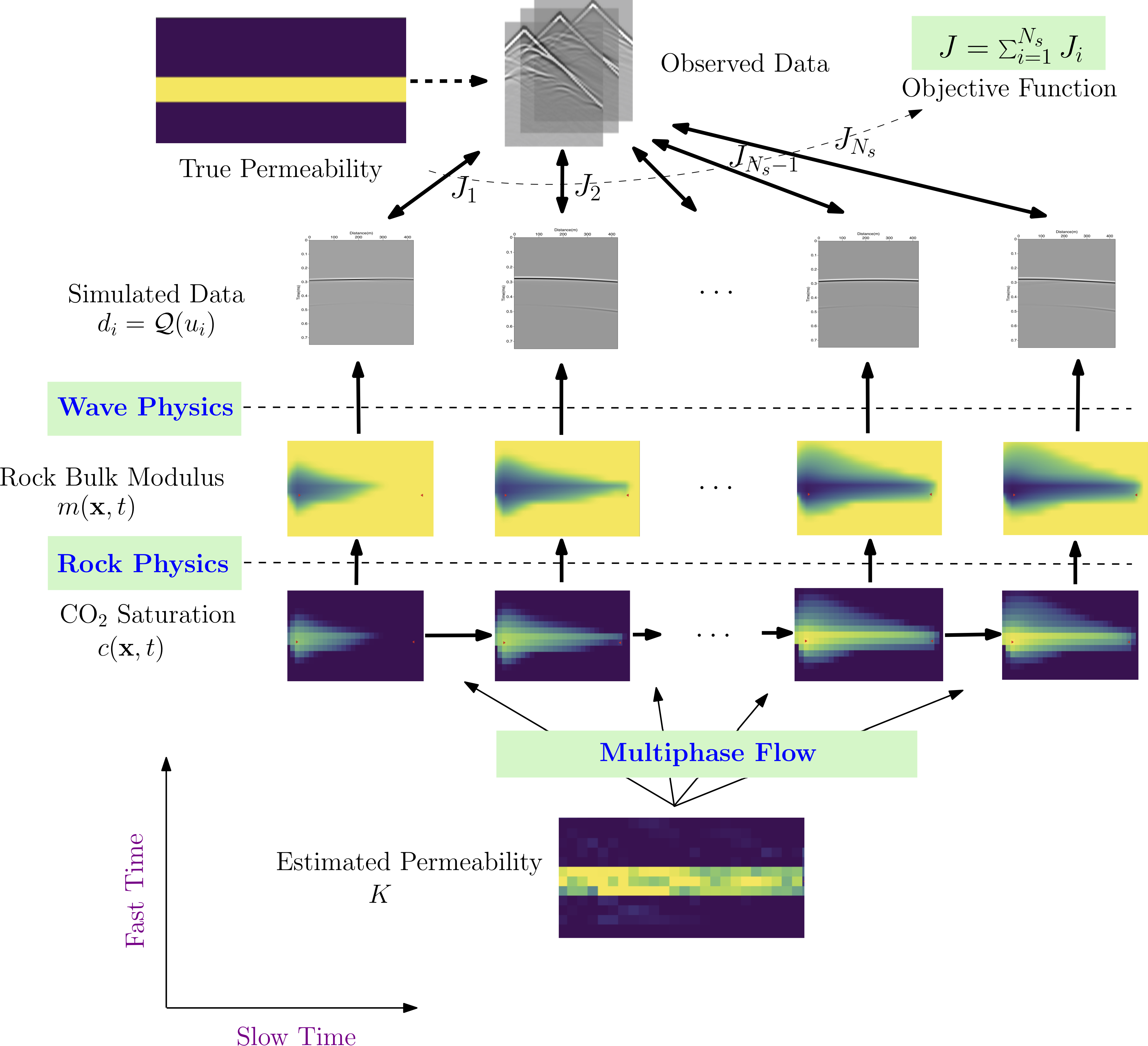
This approach is named physics constrained learning and has been used to develop FwiFlow.jl, a package for elastic full waveform inversion for subsurface flow problems. The physical equation is nonlinear, the discretization is implicit, and thus it must be solved using the Newton-Raphson method.