MPI Benchmarks
The purpose of this section is to present the distributed computing capability of ADCME via MPI. With the MPI operators, ADCME is well suited to parallel implementations on clusters with very large numbers of cores. We benchmark individual operators as well as the gradient calculation as a whole. Particularly, we use two metrics for measuring the scaling of the implementation:
- weak scaling, i.e., how the solution time varies with the number of processors for a fixed problem size per processor.
- strong scaling, i.e., the speedup for a fixed problem size with respect to the number of processors, and is governed by Amdahl's law.
For most operators, ADCME is just a wrapper of existing third-party parallel computing software (e.g., Hypre). However, for gradient back-propagation, some functions may be missing and are implemented at our own discretion. For example, in Hypre, distributed sparse matrices split into multiple stripes, where each MPI rank owns a stripe with continuous row indices. In gradient back-propagation, the transpose of the original matrix is usually needed and such functionalities are missing in Hypre as of September 2020.
The MPI programs are verified with serial programs. Note that ADCME uses hybrid parallel computing models, i.e., a mixture of multithreading programs and MPI communication; therefore, one MPI processor may be allocated multiple cores.
Transposition
Matrix transposition is an operator that are common in gradient back-propagation. For example, assume the forward computation is ($x$ is the input, $y$ is the output, and $A$ is a matrix)
\[y(\theta) = Ax(\theta) \tag{1}\]
Given a loss function $L(y)$, we have
\[\frac{\partial L(y(x))}{\partial x} = \frac{\partial L(y)}{\partial y}\frac{\partial y(x)}{\partial x} = \frac{\partial L(y)}{\partial y} A\]
Note that $\frac{\partial L(y)}{\partial y}$ is a row vector, and therefore,
\[\left(\frac{\partial L(y(x))}{\partial x}\right)^T = A^T \left(\frac{\partial L(y)}{\partial y} \right)^T\]
requires a matrix vector multiplication, where the matrix is $A^T$.
Given that Equation 1 is ubiquitous in numerical PDE schemes, a distributed implementation of parallel transposition is very important.
ADCME uses the same distributed sparse matrix representation as Hypre. In Hypre, each MPI processor own a set of rows of the whole sparse matrix. The rows have continuous indices. To transpose the sparse matrix in a parallel environment, we first split the matrices in each MPI processor into blocks and then use MPI_Isend/MPI_Irecv to exchange data. Finally, we transpose the matrices in place for each block. Using this method, we obtained a CSR representation of the transposed matrix.
![]()
The following results shows the scalability of the transposition operator of mpi_SparseTensor. In the plots, we show the strong scaling for a fixed matrix size of $25\text{M} \times 25\text{M}$ as well as the weak scaling, where each MPI processor owns $300^2=90000$ rows.
| Strong Scaling | Weak Scaling |
|---|---|
Poisson's Equation
This example presents the overhead of ADCME MPI operators when the main computation is carried out through a third-party library (Hypre). We solve the Poisson's equation
\[\nabla \cdot (\kappa(x, y) \nabla u(x,y)) = f(x, y), (x,y) \in \Omega \quad u(x,y) = 0, (x,y) \in \partial \Omega\]
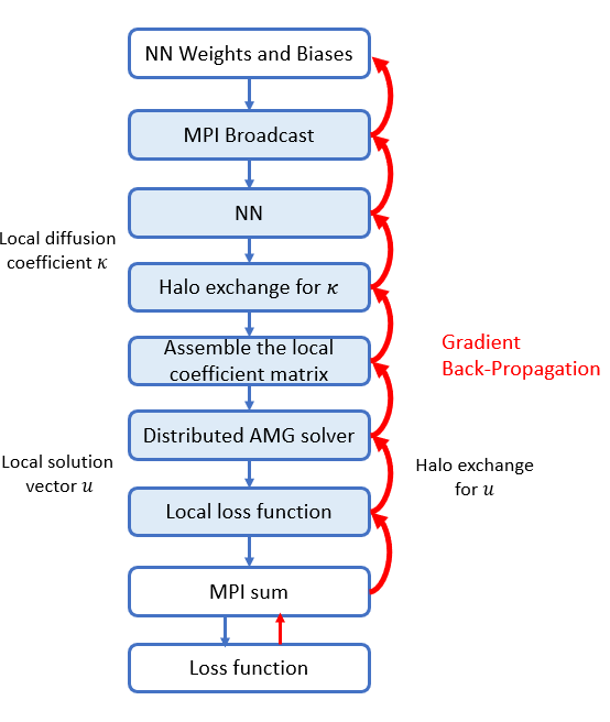
Here $\kappa(x, y)$ is approximated by a neural network $\kappa_\theta(x,y) = \mathcal{NN}_\theta(x,y)$, and the weights and biases $\theta$ are broadcasted from the root processor. We express the numerical scheme as a computational graph is:
The domain decomposition is as follows:

The domain $[0,1]^2$ is divided into $N\times N$ blocks, and each block contains $n\times n$ degrees of freedom. The domain is padded with boundary nodes, which are eliminated from the discretized equation. The grid size is
\[h = \frac{1}{Nn+1}\]
We use a finite difference method for discretizing the Poisson's equation, which has the following form
\[\begin{aligned}(\kappa_{i+1, j}+\kappa_{ij})u_{i+1,j} + (\kappa_{i-1, j}+\kappa_{ij})u_{i-1,j} &\\ + (\kappa_{i,j+1}+\kappa_{ij})u_{i,j+1} + (\kappa_{i, j-1}+\kappa_{ij})u_{i,j-1} &\\ -(\kappa_{i+1, j}+\kappa_{i-1, j}+\kappa_{i,j+1}+\kappa_{i, j-1}+4\kappa_{ij})u_{ij} &\\ = 2h^2f_{ij} \end{aligned}\]
We show the strong scaling with a fixed problem size $1800 \times 1800$ (mesh size, which implies the matrix size is around 32 million). We also show the weak scaling where each MPI processor owns a $300\times 300$ block. For example, a problem with 3600 processors has the problem size $90000\times 3600 \approx 0.3$ billion.
Weak Scaling
We first consider the weak scaling. The following plots shows the runtime for forward computation as well as gradient back-propagation.
| Speedup | Efficiency |
|---|---|
 |  |
There are several important observations:
- By using more cores per processor, the runtime is reduced significantly. For example, the runtime for the backward is reduced to around 10 seconds from 30 seconds by switching from 1 core to 4 cores per processor.
- The runtime for the backward is typically less than twice the forward computation. Although the backward requires solve two linear systems (one of them is in the forward computation), the AMG linear solver in the back-propagation may converge faster, and therefore costs less than the forward.
Additionally, we show the overhead, which is defined as the difference between total runtime and Hypre linear solver time, of both the forward and backward calculation.
| 1 Core | 4 Cores |
|---|---|
 | 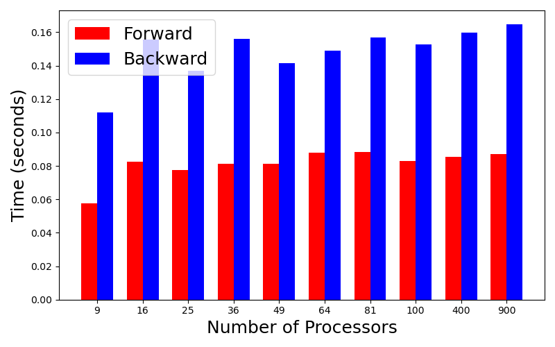 |
We see that the overhead is quite small compared to the total time, especially when the problem size is large. This indicates that the ADCME MPI implementation is very effective.
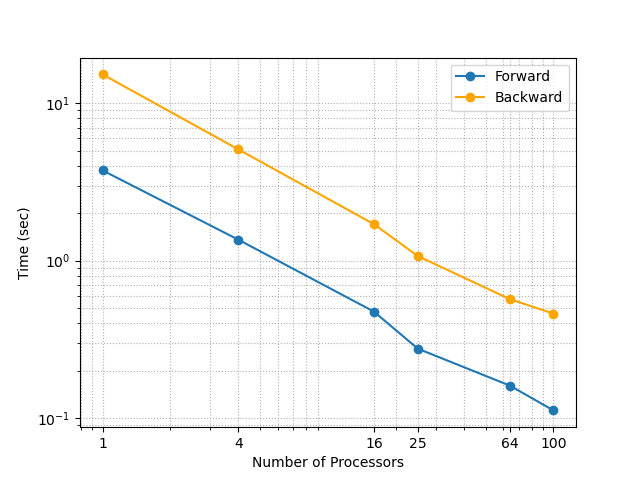
Strong Scaling
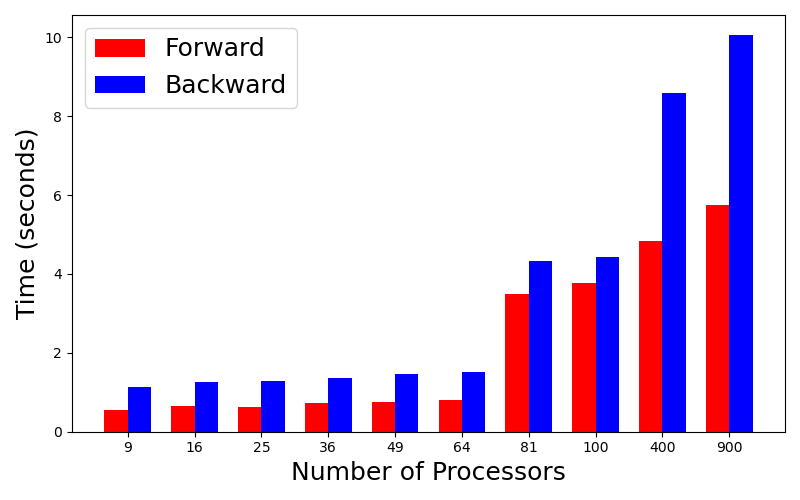
Now we consider the strong scaling. In this case, we fixed the whole problem size and split the mesh onto different MPI processors. The following plots show the runtime for the forward computation and the gradient back-propagation
| Forward | Bckward |
|---|---|
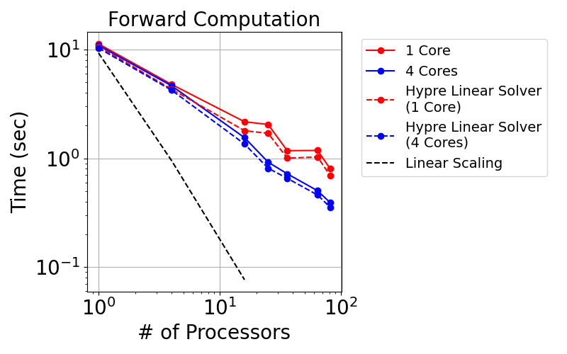 |  |
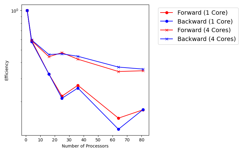
The following plots show the speedup and efficiency
| 1 Core | 4 Cores |
|---|---|
 |  |
We can see that the 4 cores have smaller runtime compared to 1 core.
Interested readers can go to here for implementations. To compile the codes, make sure that MPI and Hypre is available (see install_openmpi and install_hypre) and run the following script:
using ADCME
change_directory("ccode/build")
ADCME.cmake()
ADCME.make()
Acoustic Seismic Inversion
In this example, we consider the acoustic wave equation with perfectly matched layer (PML). The governing equation for the acoustic equation is
\[\frac{\partial^2 u}{\partial t^2} = \nabla \cdot (c^2 \nabla u)\]
where $u$ is the displacement, $f$ is the source term, and $c$ is the spatially varying acoustic velocity.
In the inverse problem, only the wavefield $u$ on the surface is observable, and we want to use this information to estimate $c$. The problem is usually ill-posed, so regularization techniques are usually used to constrain $c$. One approach is to represent $c$ by a deep neural network
\[c(x,y) = \mathcal{NN}_\theta(x,y)\]
where $\theta$ is the neural network weights and biases. The loss function is formulated by the square loss for the wavefield on the surface.
| Model $c$ | Wavefield |
|---|---|
 |  |
To implement an MPI version of the acoustic wave equation propagator, we use mpi_halo_exchange, which is implemented using MPI and performs the halo exchange mentioned in the last example for both wavefields and axilliary fields. This function communicates the boundary information for each block of the mesh. The following plot shows the computational graph for the numerical simulation of the acoustic wave equation

The following plot shows the strong scaling and weak scaling of our implementation. Each processor consists of 32 processors, which are used at the discretion of ADCME's backend, i.e., TensorFlow. The strong scaling result is obtained by using a $1000\times 1000$ grid and 100 times steps. For the weak scaling result, each MPI processor owns a $100\times 100$ grid, and the total number of steps is 2000. It is remarkable that even though we increase the number of processors from 1 to 100, the total time only increases 2 times in the weak scaling.
| Strong Scaling | Weak Scaling |
|---|---|
 |  |
We also show the speedup and efficiency for the strong scaling case. We can achieve more than 20 times acceleration by using 100 processors (3200 cores in total) and the trend is not slowing down at this scale.

Elastic Seismic Inversion
In the last example, we consider the elastic wave equation
\[\begin{aligned} \rho \frac{\partial v_i}{\partial t} &= \sigma_{ij,j} + \rho f_i \\ \frac{\partial \sigma_{ij}}{\partial t} &= \lambda v_{k, k} + \mu (v_{i,j}+v_{j,i}) \end{aligned}\tag{2}\]
where $v$ is the velocity, $\sigma$ is the stress tensor, $\rho$ is the density, and $\lambda$ and $\mu$ are the Lamé constants. Similar to the acoustic equation, we use the PML boundary conditions and have observations on the surface. However, the inversion parameters are now spatially varying $\rho$, $\lambda$ and $\mu$.

As an example, we approximate $\lambda$ by a deep neural network
\[\lambda(x,y) = \mathcal{NN}_\theta(x,y)\]
and the other two parameters are kept fixed.
We use the same geometry settings as the acoustic wave equation case. Note that elastic wave equation has more state variables as well as auxilliary fields, and thus is more memory demanding. The huge memory cost calls for a distributed framework, especially for large-scale problems.
Additionally, we use fourth-order finite difference scheme for discretizing Equation 2. This scheme requires us to exchange two layers on the boundaries for each block in the mesh. This data communication is implemented using MPI, i.e., mpi_halo_exchange2.
The following plots show the strong and weak scaling. Again, we see that the weak scaling of the implementation is quite effective because the runtime increases mildly even if we increase the number of processors from 1 to 100.
| Strong Scaling | Weak Scaling |
|---|---|
 |  |
The following plots show the speedup and efficiency for the strong scaling. We can achieve more than 20 times speedup when using 100 processors. 