Inverse Modeling Recipe
Here is a tip for inverse modeling using ADCME.
Forward Modeling
The first step is to implement your forward computation in ADCME. Let's consider a simple example. Assume that we want to compute a transformation from $\{x_1,x_2, \ldots, x_n\}$ to $\{f_\theta(x_1), f_\theta(x_2), \ldots, f_\theta(x_n)\}$, where
\[f_\theta(x) = a_2\sigma(a_1x+b_1)+b_2\quad \theta=(a_1,b_2,a_2,b_2)\]
The value $\theta=(1,2,3,4)$. We can code the forward computation as follows
using ADCME
θ = constant([1.;2.;3.;4.])
x = collect(LinRange(0.0,1.0,10))
f = θ[3]*sigmoid(θ[1]*x+θ[2])+θ[4]

sess = Session(); init(sess)
f0 = run(sess, f)
We obtained
10-element Array{Float64,1}:
 6.6423912339336475
 6.675935315969742
 6.706682200447601
 6.734800968378825
 6.7604627001561575
 6.783837569144308
 6.805092492614008
 6.824389291376896
 6.841883301751329
 6.8577223804673
Inverse Modeling
Assume that we want to estimate the target variable $\theta$ from observations $\{f_\theta(x_1), f_\theta(x_2), \ldots, f_\theta(x_n)\}$. The inverse modeling is split into 6 steps. Follow the steps one by one
Step 1: Mark the target variable as
placeholder. That is, we replaceθ = constant([1.;2.;3.;4.])byθ = placeholder([1.;2.;3.;4.]).Step 2: Check that the loss is zero given true values. The loss function is usually formulated so that it equals zero when we plug the true value to the target variable.
You should expect
0.0using the following codes.
using ADCME
θ = placeholder([1.;2.;3.;4.])
x = collect(LinRange(0.0,1.0,10))
f = θ[3]*sigmoid(θ[1]*x+θ[2])+θ[4]
loss = sum((f - f0)^2)
sess = Session(); init(sess)
@show run(sess, loss)- Step 3: Use
lineviewto visualize the landscape. Assume the initial guess is $\theta_0$, we can use thelineviewfunction fromADCMEKit.jlpackage to visualize the landscape from $\theta_0=[0,0,0,0]$ to $\theta^*$ (true value). This gives us early confidence on the correctness of the implementation as well as the difficulty of the optimization problem. You can also usemeshview, which shows a 2D landscape but is more expensive to evaluate.
using ADCME
using ADCMEKit
θ = placeholder([1.;2.;3.;4.])
x = collect(LinRange(0.0,1.0,10))
f = θ[3]*sigmoid(θ[1]*x+θ[2])+θ[4]
loss = sum((f - f0)^2)
sess = Session(); init(sess)
@show run(sess, loss)
lineview(sess, θ, loss, [1.;2.;3.;4.], zeros(4)) # or meshview(sess, θ, loss, [1.;2.;3.;4.])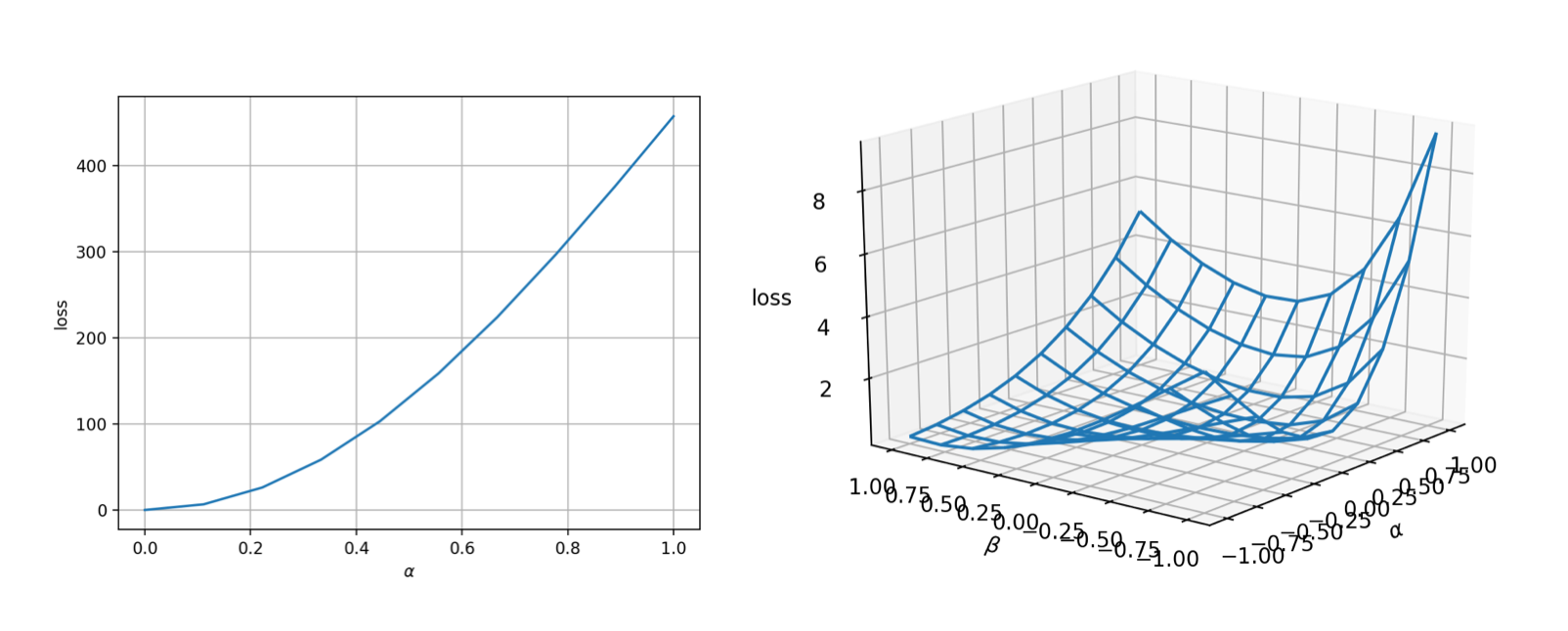
The landscape is very nice (convex and smooth)! That means the optimization should be very easy.
- Step 4: Use
gradviewto check the gradients.ADCMEKit.jlalso providesgradviewwhich visualizes the gradients at arbitrary points. This helps us to check whether the gradient is implemented correctly.
using ADCME
using ADCMEKit
θ = placeholder([1.;2.;3.;4.])
x = collect(LinRange(0.0,1.0,10))
f = θ[3]*sigmoid(θ[1]*x+θ[2])+θ[4]
loss = sum((f - f0)^2)
sess = Session(); init(sess)
@show run(sess, loss)
lineview(sess, θ, loss, [1.;2.;3.;4.], zeros(4)) # or meshview(sess, θ, loss, [1.;2.;3.;4.])
gradview(sess, θ, loss, zeros(4)) You should get something like this:
- Step 5: Change
placeholdertoVariableand perform optimization! We use L-BFGS-B optimizer to solve the minimization problem. A useful trick is to multiply the loss function by a large scalar so that the optimizer does not stop early (or reduce the tolerance).
using ADCME
using ADCMEKit
θ = Variable(zeros(4))
x = collect(LinRange(0.0,1.0,10))
f = θ[3]*sigmoid(θ[1]*x+θ[2])+θ[4]
loss = 1e10*sum((f - f0)^2)
sess = Session(); init(sess)
BFGS!(sess, loss)
run(sess, θ)
You should get
4-element Array{Float64,1}:
 1.0000000000008975
 2.0000000000028235
 3.0000000000056493
 3.999999999994123
That's exact what we want.
- Step 6: Last but not least, repeat step 3 and step 4 if you get stuck in a local minimum. Scrutinizing the landscape at the local minimum will give you useful information so you can make educated next step!
Debugging
Sensitivity Analysis
When the gradient test fails, we can perform unit sensitivity analysis. The idea is that given a function $y = f(x_1, x_2, \ldots, x_n)$, if we want to confirm that the gradients $\frac{\partial f}{\partial x_i}$ is correctly implemented, we can perform 1D gradient test with respect to a small perturbation $\varepsilon_i$:
\[y(\varepsilon_i) = f(x_1, x_2, \ldots, x_i + \varepsilon_i, \ldots, x_n)\]
or in the case you are not sure about the scale of $x_i$,
\[y(\varepsilon_i) = f(x_1, x_2, \ldots, x_i (1 + \varepsilon_i), \ldots, x_n)\]
As an example, if we want to check whether the gradients for sigmoid is correctly backpropagated in the above code, we have
using ADCME
using ADCMEKit
ε = placeholder(1.0)
θ = constant([1.;2.;3.;4.])
x = collect(LinRange(0.0,1.0,10))
f = θ[3]*sigmoid(θ[1]*x+θ[2] + ε)+θ[4]
loss = sum((f - f0)^2)
sess = Session(); init(sess)
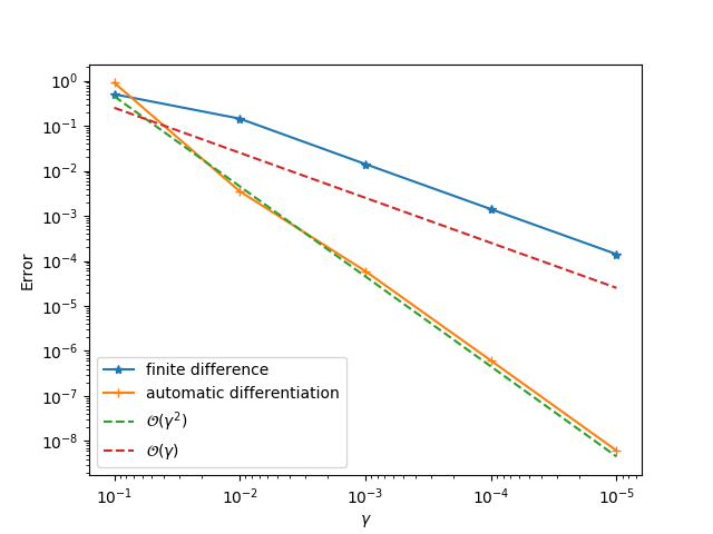
gradview(sess, ε, loss, 0.01)We will see a second order convergence for the automatic differentiation method while a first order convergence for the finite difference method. The principle for identifying problematic operator is to go from downstream operators to top stream operators in the computational graph. For example, given the computational graph
\[f_1\rightarrow f_2 \rightarrow \cdots \rightarrow f_i \rightarrow f_{i+1} \rightarrow \ldots \rightarrow f_n\]
If we conduct sensitivity analysis for $f_i:o_i \mapsto o_{i+1}$, and find that the gradient is wrong, then we can infer that at least one of the operators in the downstream $f_i \rightarrow f_{i+1} \rightarrow \ldots \rightarrow f_n$ has problematic gradients.
Check Your Training Data
Sometimes it is also useful to check your training data. For example, if you are working with numerical schemes, check whether your training data are generated from reasonable physical parameters, and whether or not the numerical schemes are stable.
Local Minimum
To check whether or not the optimization converged to a local minimum, you can either check meshview or lineview. However, these functions only give you some hints and you should only rely solely on their results. A more reliable check is to consider gradview. In principle, if you have a local minimum, the gradient at the local minimum should be zero, and therefore the finite difference curve should also have second order convergence.