Study on Optimizers
When working with BFGS/LBFGS, there are some important aspects of the algorithm, which affect the convergence of the optimizer.
- BFGS approximates the Hessian or the inverse Hessian matrix. LBFGS, instead, stores a limited set of vectors and does not explicitly formulate the Hessian matrices. The Hessian matrix solve is approximated using recursions on vector vector production.
- Both BFGS and LBFGS deploy a certain kind of line search strategies. For example, the Hager-Zhang and More-Thuente are two commonly used strategies. These linesearch algorithms require evaluating gradients in each line search step. This means we need to frequently do gradient back-propagation, which may be quite expensive. We instead employ a backtracking strategy, which requires evaluating forward computation only.
- Initial guess of the line search algorithm. We found that the following initial guess is quite effective for our problems:
\[\alpha=\min\{100\alpha_0, 10\}\]
Here $\alpha_0$ is the line search step size for the last step (for the first step, $\alpha=1$ is used). Using this choice, we found that in a typical line search step, only 1~3 evaluations of the loss function is needed. - Stopping criterion in line search algorithms. The algorithm backtracks until a certain set of condition is met. Typically the Wolfe condition, the Armijo curvature rule, or the strong Wolfe conditions are used. Note that these criterion require gradient information, and we want to avoid calculating extra gradients during linesearch. Therefore, we use the following sufficient decrease condition
\[\phi(\alpha) \leq \phi(0) + c_1 \alpha \phi'(0)\]
Here $c_1=10^{-4}$.
One interesting observation is that if we apply BFGS/LBFGS directly, we usually cannot make any progress. There are many reasons for this phenomenon:
- The initial guess for the neural network is far away from optimal, and quasi-Newton methods usually do not work well in this regime.
- The approximate Hessian is quite different from the true one. The estimated search direction may deviate from the optimal one too much.
First-order methods, such as Adam optimizer, usually does not suffer from these difficulties. Therefore, one solution to this problem is via "warm start" by running a first order optimizer (Adam) for a few iterations. Additionally, for BFGS, we can build Hessian approximations while we are running the Adam optimizer. In this way, we can use the historic information as much as possible.
Our algorithm is as follows (BFGS+Adam+Hessian):
Run the Adam optimizer for the first few iterations, and build the approximate Hessian matrix at the same time. That is, in each iteration, we update an approximate Hessian $B$ using
$B_{k+1} = \left(I - \frac{s_k y_k^T}{y_k^Ts_k}\right)B_k\left(I - \frac{ y_ks_k^T}{y_k^Ts_k}\right) + \frac{s_ks_k^T}{y_k^Ts_k}$
Here $y_k = \nabla f(x_{k+1}) - \nabla f(x_{k}), s_k = x_{k+1}-x_k, B_0 = I$. Note $B_k$ is not used in the Adam optimizer.
Run the BFGS optimizer and use the last Hessian matrix $B_k$ built in Step 1 as the initial guess.
We compare our algorithm with those without approximated Hessian (BFGS+Adam) or warm start (BFGS). Additionally, we also compare our algorithm with LBFGS counterparts.
In the test case II and III, a physical field, $f$, is approximated using deep neural networks, $f_\theta$, where $\theta$ is the weights and biases. The neural network maps coordinates to a scalar value. $f_\theta$ is coupled with a DAE:
\[F(u', u, Du, D^2u, \ldots ;f_\theta) = 0 \tag{1}\]
Here $u'$ represents the time derivative of $u$, and $Du$, $D^2u$, $\ldots$ are first-, second-, $\ldots$ order spatial gradients. Typically we can observe $u$ on some discrete points $\{\mathbf{x}_k\}_{k\in \mathcal{I}}$. To train the neural network, we consider the following optimization problem
\[\min_\theta \sum_{k\in \mathcal{I}} (u(\mathbf{x}_i) - u_\theta(\mathbf{x}_i))\]
Here $u_\theta$ is the solution from Eq. 1.
Test Case I
In the first case, we train a 4 layer network with 20 neurons per layer, and tanh activation functions. The data set is $\{x_i, sin(x_i)\}_{i=1}^{100}$, where $x_i$ are randomly generated from $\mathcal{U}(0,1)$. The neural network $f_\theta$ is trained by solving the following optimization problem:
\[\min_\theta \sum_{i=1}^{100} (\sin(x_i) - f_\theta(x_i))^2\]
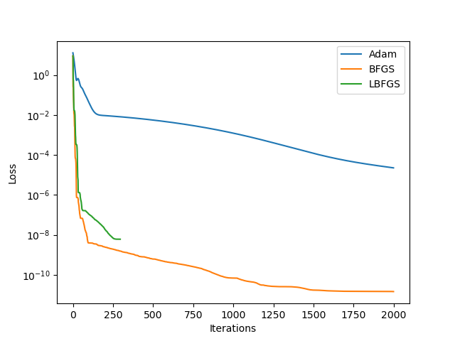
The neural network is small, and thus we can use BFGS/LBFGS to train. In fact, the following plot shows that BFGS/LBFGS is much more accurate and effective than the commonly used Adam optimizer. Considering the wide range of computational engineering applications, where a small neural network is sufficient, this result implies that BFGS/LBFGS for training neural networks should receive far more attention than what it does nowadays.
Also, in many applications, the major runtime is doing physical simulations instead of updating neural network parameters or approximate Hessian matrices, these "expensive" BFGS/LBFGS optimization algorithms should be considered a good way to leverage as much history information as possible, so as to reduce the total number of iterations (simulations).
Test Case II
In this test case, we consider solving a Poisson's equation in this post.
The exact $\kappa$ and the corresponding solution $u$ is shown below

We run different optimization algorithms and obtain the following loss function profiles. We see that BFGS/LBFGS without Adam warm start terminates early. BFGS in general has much better accuracy than LBFGS. An extra benefit of BFGS+Adam+Hessian compared to BFGS+Adam is that we can achieve much better accuracy.
| Loss Function | Zoom-in View |
|---|---|
 |  |
We also show the mean squared error for $\kappa$, which confirms that BFGS+Adam+Hessian achieves the best test error. The error is calculated using the formula
\[\frac{1}{n} (\kappa_{\text{true}}(\textbf{x}_i) - \kappa_\theta(\textbf{x}_i))^2\]
Here $\textbf{x}_i$ is defined on Gauss points.
| Algorithm | Adam | BFGS+Adam+Hessian | BFGS+Adam | BFGS | LBFGS+Adam | LBFGS |
|---|---|---|---|---|---|---|
| MSE | 0.013 | 1.00E-11 | 1.70E-10 | 1.10E+04 | 0.00023 | 97000 |
Test Case III
In the last example, we consider the linear elasticity. The problem description can be found here.
We fix the random seed for neural network initialization and run different optimization algorithms. The initial guess for the Young's modulus and the reference one are shown in the following plot

The corresponding velocity and stress fields are

We perform the optimization using different algorithms. In the case where Adam is used as warm start, we run Adam optimization for 50 iterations. We run the optimization for at most 500 iterations (so there is at most 500 evaluations of gradients) The loss function is shown below

We see that BFGS+Adam+Hessian achieves the smallest loss functions among all algorithms. We also show the MSE for $E$, i.e., $\frac{1}{n} (E_{\text{true}}(\textbf{x}_i) - E_\theta(\textbf{x}_i))^2$, where $\textbf{x}_i$ is defined on Gauss points.
| Algorithm | Adam | BFGS+Adam+Hessian | BFGS+Adam | BFGS | LBFGS+Adam | LBFGS |
|---|---|---|---|---|---|---|
| MSE | 0.0033 | 1.90E-07 | 4.00E-06 | 6.20E-06 | 0.0031 | 0.0013 |
This confirms that BFGS+Adam+Hessian indeed generates a much more accurate result.
We also compare the results for the BFGS+Adam+Hessian and Adam algorithms:

We see the Adam optimizer achieves reasonable result but is challenging to deliver high accurate estimation within 500 iterations.